We'll use the famous Simulink Real Time Execution S-function by Guy Rouleau, published in the MATLAB Central at the address http://www.mathworks.com/matlabcentral/fileexchange/21908-simulink%C2%AE-real-time-execution.

The code bundle coming with this chapter already contains the RealTimeSlower folder with all the needed files for Windows (32 and 64 bit) and UNIX/Linux (64 bit); we only have to add that folder to our MATLAB path, as explained in Chapter 2, Creating a Model.

The Simulink Library Browser will now have a new item: the Soft Real Time block under the Soft Real Time Lib blockset. This block is the one that does the trick for us, that is, syncs Simulink to the system clock.

Let's make a copy of the cruise controller model we did in Chapter 2, Creating a Model, and save it to the current working folder as cruise_control_external_msfun.slx.

The calibration constants Kp and Ki have to be set to the values we found in Chapter 3, Simulating a Model. They were 0.4 and 0.002, respectively. Let's set them now:

Kp = 0.4;
Ki = 0.002;

Save the workspace as cruise_control_external.mat. We'll add the load('cruise_control_external.mat') command to the model's PreLoadFcn callback too, as shown in Chapter 2, Creating a Model.

Then we'll open the Model configuration parameters window (shortcut: Ctrl + E) and set the fixed-step solver ode1 (Euler), with a Fixed-step size of 0.1 seconds. The simulation Stop time should be set to inf, since we want the simulation to run indefinitely until we stop it.

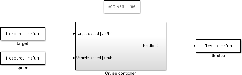
Finally, instead of the root-level input and output ports, we'll use the blocks we just made, along with the Soft Real Time block:

The prepared cruise controller model should look like the following screenshot:

Don't forget to do a model update (shortcut: Ctrl + D) as a little check.

Now we're ready to have some fun!

With the directions we had at the beginning of this chapter, we'll start the external application inside the same folder as the model, and set these file paths:

Before hitting the Run button in Simulink, hit the Run button in the target application first! Otherwise, our filesource_msfun blocks will recognize that the input files don't exist (they're created by the application as soon as its Run button is clicked) and throw an error. The application is less picky: the files, if they don't exist, will be automatically created.

Now we can move the Target speed slider, and the cruise controller will try to match it through the throttle. The simulated car will react to the throttle input, and the vehicle speed will be painted with a blue line on the application's Speed graph. The application will update the Throttle and the Gear graphs too.

An example is presented in the following screenshot:

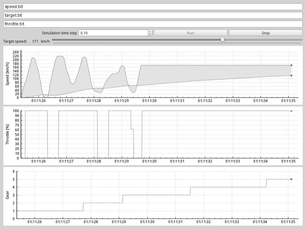
Isn't it awesome to see our Simulink cruise controller model interacting with something so different?

When we're tired of investigating how fast the car can go, measuring the 0-100 km/h time, and frantically moving the slider trying to get the Euler solver to diverge, you can stop the simulation and the application by clicking on the provided Stop buttons.