
With what we've learned so far, we're ready to develop a simple mathematical model of a real car in order to test and fine-tune the controller in a closed-loop simulation.
Luckily enough, a lot of technical detail is available nowadays on almost every car. The author likes the Alfa Romeo 147 GTA a lot, so the choice is made.
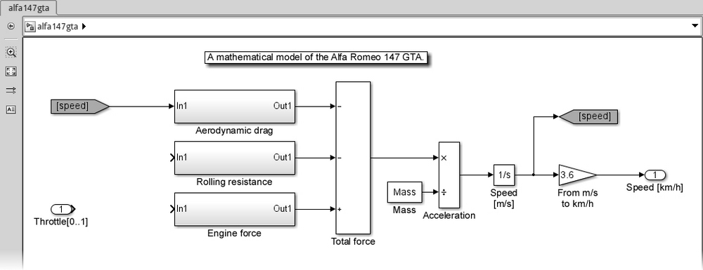
Open a new Simulink model and save it as alfa147gta.slx. The model will have one input (the throttle, coming from the cruise controller) and one output (the car's speed, going to the cruise controller).
We're interested only in the longitudinal speed (a car going straight on a flat ground), and we assume the gearbox to be ideal (shifting gears in no time).
How do we compute the speed?
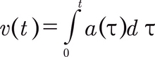
We know that the car's speed is the integral of the acceleration in time:
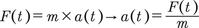
Newton's second law reminds us that the acceleration is proportional to the total force applied on the car, with the mass m being the factor:
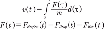
Since we're building a simplified model, we'll consider only the following three main forces:
- The engine force FEngine, generated by the fuel burning in the engine
- The aerodynamic drag FDrag, generated by the car moving in the air (that is, a viscous fluid)
- The rolling resistance FRes, the sum of all the rolling frictions that oppose the movement
Putting it all together, we have:
The mass being a constant, we can declare it in the workspace right away. The Alfa 147 GTA weighs 1360 kg, so we'll enter the following command in MATLAB's main window:
Mass = 1360;
Let's make the relevant blocks in the root system. Open Library Browser and drag three Subsystem blocks into the model (one for each force applied) from the Ports & Subsystems blockset; one Add block and one Divide block from the Math Operations blockset; one Integrator block from the Continuous blockset; and one Constant block from the Sources blockset for the mass.
Since we'll be working with the international metric system inside this model, we'll put a Gain block too (from the Math Operations blockset) before the output, to convert the speed unit from m/s to the one used by the cruise controller, km/h.
Rename the Subsystem blocks to Aerodynamic drag, Rolling Resistance, and Engine Force, and align them vertically.
Double-click on the Add block and edit the list of signs; we need three inputs, only one positive (the engine force). Let's keep the positive input as the last; the list of signs should be --+.
Double-click on the Constant block and set its Constant value parameter to Mass (the variable we just created in the workspace).
The same must be done for the Gain block, setting the Gain to 3.6 in order to convert from m/s to km/h.
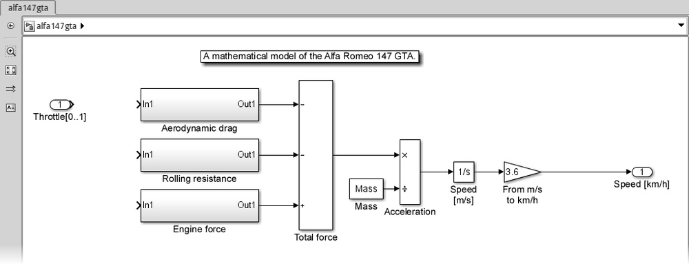
After putting a brief note, connecting the blocks following the above formulas, and renaming the blocks, we should have our model as shown in the following screenshot:
We still need to compute the forces. We'll start with the drag and the rolling resistance first, since they're simpler; then we'll build the algorithm calculating the engine force.
The aerodynamic drag force, whose effect is evident at high vehicle speeds, can be calculated with the drag equation as follows:

KDrag is a constant for the car, made of:
- The air density ρ, at 20 °C and 101.325 kPa equals to 1.2041 kg/m3
- The drag coefficient CD, which is 0.32 for the 147 GTA
- The frontal area A, approx. 2.2 m2
Let's declare it in the workspace with the following command:
Kdrag = 0.5 * 1.2041 * 0.32 * 2.2;
Since the vehicle speed needs to be an input of the block, we're adding a Goto and From block from the Signal Routing blockset to the root block.
Tip
The Goto and From blocks can avoid drawing a connection between two or more subsystems and are extremely helpful to avoid cluttering the view. It's a common practice in the automotive industry to use them instead of connecting input and output ports directly to the subsystems implementing the logic. When the system becomes too complex and there are many tags, it's helpful to assign the same foreground/background color to matching Goto and From blocks. This can be done by right-clicking on the block and using the Format menu option.
Open both and use the same tag: speed. It's suggested to hide their names. Be careful to connect the Goto block at the end of the integrator—we want the speed in m/s, not in km/h.
The root system should be looking like the following screenshot:
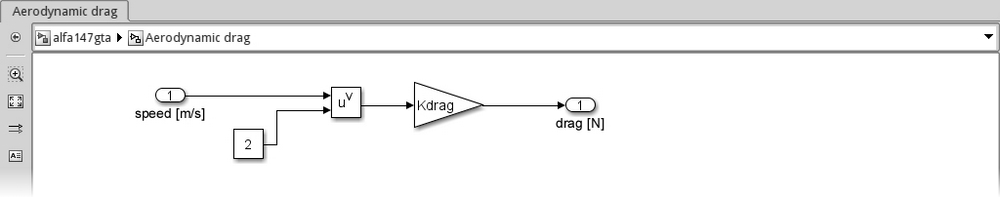
Inside the Aerodynamic drag subsystem, we'll implement the drag equation with one Gain block, one Math function block (both from Simulink | Math Operations), and one Constant block (from Simulink | Sources).
We'll use Kdrag as the Gain parameter for the Gain block and select the pow function in the Math function block (double-click and set the Function drop-down list to pow). A second input will appear; it is the exponential to apply; we'll connect it to the Constant block and set its Constant value parameter to 2.
Finally, we'll rename and connect the input and output ports, the input being the speed (in m/s) and the output being the drag force (in N). After making the connections, the subsystem should look like the following:
Don't forget to copy and connect the speed Goto in the parent system to the input port.
Let's do the next step, the rolling resistance.
The rolling resistance (sometimes called rolling friction or rolling drag) is proportional to the vehicle speed. It's the main resistance at a lower speed.
It's not simple to obtain a precise formula because it involves knowledge about the tire characteristics, but we can simplify the calculations by assuming that:
- At approximately 30 m/s (100 km/h), the rolling resistance and the drag are equal
- The proportional factor is constant at other speeds
This assumption is valid for most cars.
So we can find, with v = 30 m/s, the constant KRes:
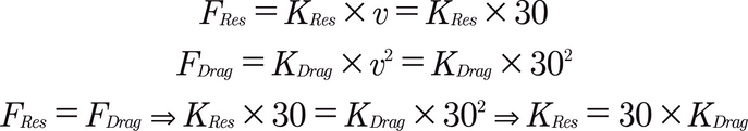
KRes being just 30 times bigger than KDrag, we don't even need to declare a new variable in the workspace.
The implementation is simple: we just put inside the Rolling resistance subsystem a Gain block set to 30*Kdrag and connect it to the input and output ports (renamed as usual). We should have this subsystem:
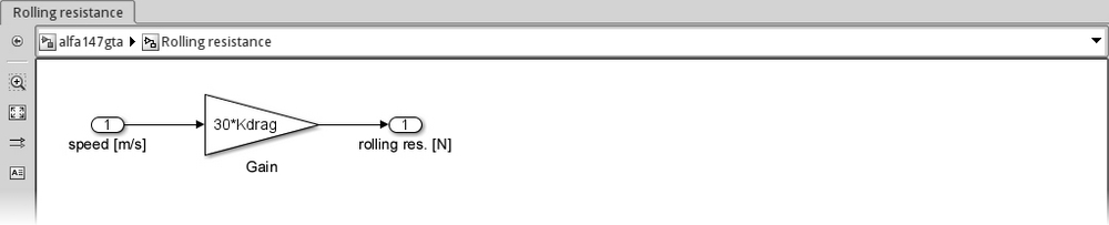
Don't forget to copy and connect the speed Goto in the parent system to the input port.
So far, so good. Now comes the hard part: the subsystem that calculates the engine force requested by the cruise controller (via the throttle input).
Every combustion engine has a characteristic torque curve (also called lug curve) that can be found in almost every technical review book. The Alfa 147 GTA shows the following one:
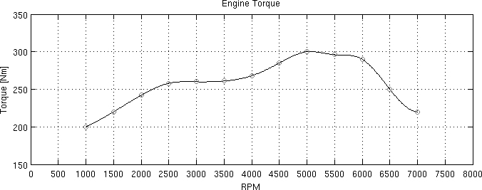
The torque in the preceding graph represents the maximum available torque τMAX (with the throttle fully open), measured at the crankshaft.
The engine and the wheels are linked together through the gearbox and the differential; the former applies a variable gear ratio KGear and the latter applies a constant final ratio KFinal.
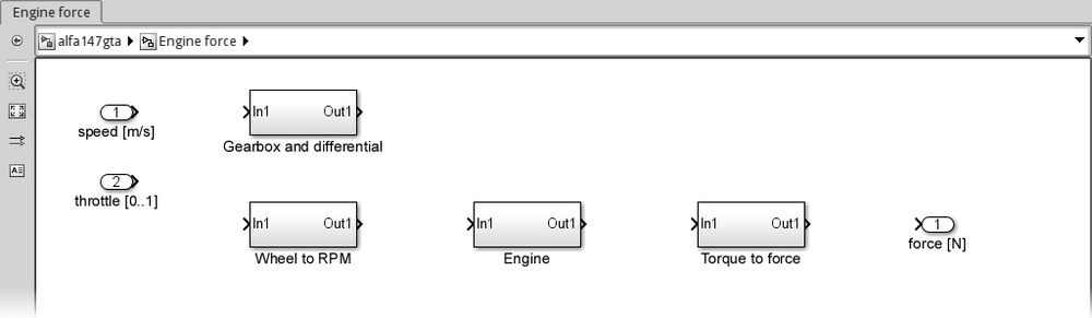
Since we have to transform the vehicle speed to engine RPM first and the engine torque to the engine force last, all taking into account the gearbox and differential combined ratios, we need to model four subsystems:
- Gearbox and differential, will output the transmission ratio at the current speed
- Wheel to RPM, will output the current RPM based on the current transmission ratio and the current speed
- Engine, will receive the throttle command and output the resulting torque at the current RPM
- Torque to force, will convert the engine torque to the force that the engine is applying on the car
Let's start by having two input ports (the vehicle speed and the throttle input), one output port (the engine force), and the four empty Subsystem blocks (found in Simulink | Ports & Subsystems) in the Engine force subsystem. The subsystem should now look like the following screenshot:
The first subsystem we'll implement is Gearbox and differential.
From the crankshaft to the wheel, the rotation is reduced twice: first in the gearbox, where the reduction ratio can be changed by upshifting/downshifting, then in the differential, which has a fixed reduction ratio.
We need to implement an automatic gearbox; the simplest is the one that chooses the gear based on the current speed and doesn't have the reverse gear.
In the following table, we'll find the Alfa 147 GTA optimal speed ranges for each gear, together with the gear ratio KGear:
|
Gear |
Speed range [km/h] |
Gear ratio |
|---|---|---|
|
1 |
< 39 |
3.500 |
|
2 |
39 – 59 |
2.235 |
|
3 |
60 – 86 |
1.520 |
|
4 |
86 – 109 |
1.156 |
|
5 |
110 – 129 |
0.971 |
|
6 |
≥ 130 |
0.818 |
The differential on the Alfa 147 GTA applies a final ratio KFinal of 3.733.
As an example: in the first gear, the engine's crankshaft is rotating 13 times (3.5*3.733) faster than the wheel axis, while in sixth gear, it's only three times (0.818*3.733) faster.
We'll put this data right now in the workspace by executing these commands:
GearRatio = [3.500 2.235 1.520 1.156 0.971 0.818];
FinalRatio = 3.733;
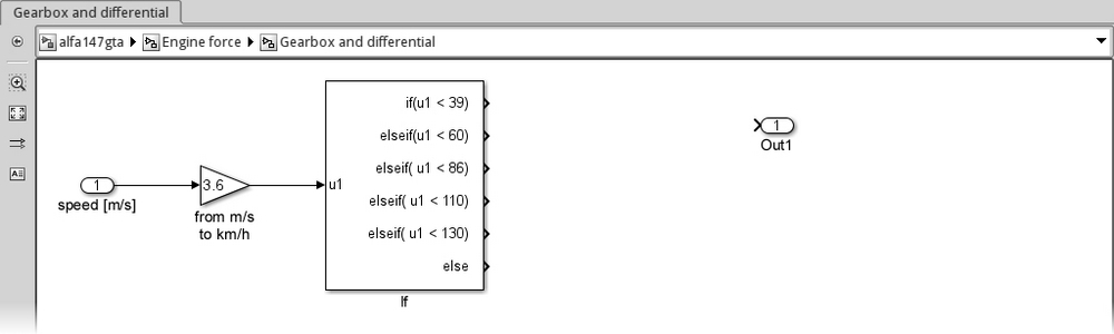
Let's build the automatic gearbox; the input is the vehicle speed in m/s, which gets converted to km/h through a Gain block with the value set to 3.6.
Then we'll use a particular construct to select the gear: an If block from the Ports & Subsystems blockset. The If block allows us to replicate exactly the C language's if()...elseif()...else construct. Opening the block parameters window reveals that we have to set the first if() condition: then we can define as many elseif() conditions as we like.
Looking at the speed ranges, it's easy to set the parameters:
- The Number of inputs will be set to
1, since we only need to evaluate the vehicle speed (the corresponding label inside the block will be u1) - The If expression will be
u1 < 39(the first gear) - The Elseif expressions elements will be
u1 < 60, u1 < 86, u1 < 110, u1 < 130(gears 2 through 5) - The Show else condition checkbox will be checked (the sixth gear)
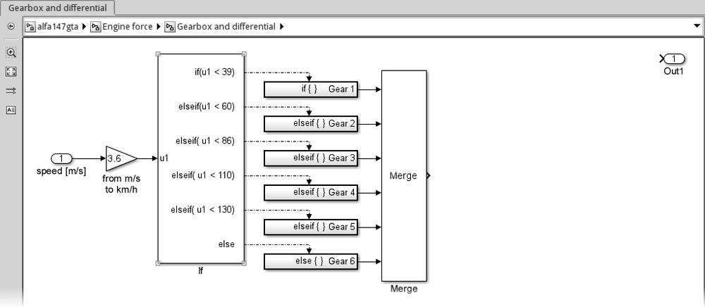
If we entered the parameters correctly, we should have the following subsystem now:
For each output of the If block, we need to put one If Action Subsystem (available in the Ports & Subsystems blockset). These subsystems must contain the code to be executed when the corresponding condition in the If block is verified (they're called conditionally executed subsystems). In our case, they'll output the chosen gear number. We don't need the input port; remove it from each one of these subsystems using a Constant block with the gear number instead.
In the following screenshot, we can see how the subsystem looks after inserting and editing the If Action Subsystem relative to the first gear and running the Simulation | Update Diagram action (the keyboard shortcut is Ctrl + D):
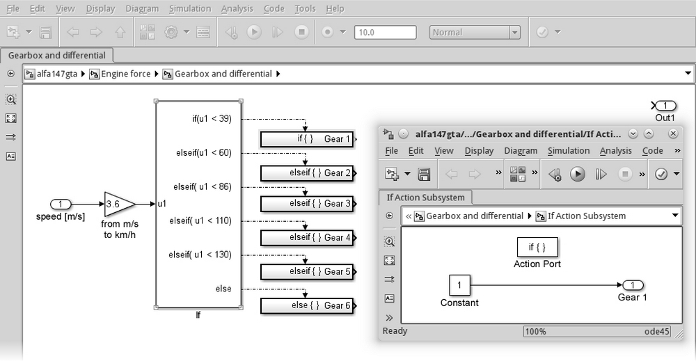
Notice that the connections between the If block and the subsystems are dotted. This means that the connection is not transporting a signal, but it's a function-call. When a condition is verified, the If block will call the subsystem connected to the corresponding port, executing its code.
We now have six possible gear values; how to put them together? We must use another particular block: the Merge block from the Signal Routing blockset. This block will instruct the connected subsystems to write their outputs to the same signal.
Let's put one Merge block into our model and open the parameters window by double-clicking on it. Since we have six subsystems, we need to set its Number of inputs parameter to 6, then connect each subsystem to one of the inputs.
The resulting model should be the one shown as follows:
Now that we have the gear, we must use it to select the gear ratio.
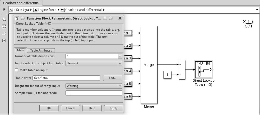
We'll use Direct Lookup Table (n-D) (from Simulink | Lookup Tables). Open the parameters window, set the Number of table dimensions parameter to 1 and the Table data parameter to GearRatio. Since the table must be accessed with a zero-based index, we must subtract one unit from the gear number coming from the Merge block.
The subsystem and the Direct Lookup Table parameters are shown in the following screenshot:
The last step is to include the final ratio due to the differential. That's easily done by putting a Gain block right before the output port (that should be renamed), and setting its Gain parameter to FinalRatio.
The final Gearbox and differential subsystem is shown in the following screenshot:
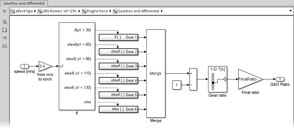
This subsystem's output will be used to convert the vehicle speed to the engine RPM, and later the engine torque to the new vehicle speed.
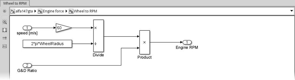
The purpose of this subsystem is to get the engine RPM using two inputs: the vehicle speed, and the combined (gear and differential) reduction ratio.
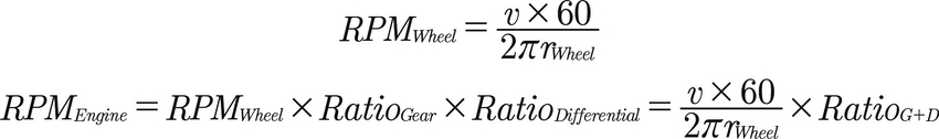
The vehicle speed v can be translated to the rotational speed of the wheel (in RPM, revolutions per minute). The RPMWheel is equal to the distance the car has traveled in 60 seconds (v*60), divided by the wheel diameter (that is, 2π times the wheel radius rWheel).
Then we know that the engine and the wheels are linked together through the gearbox and the differential. We already have their ratios; the engine's RPMEngine is equal to RPMWheel multiplied by the gear and differential ratios.
This gives us these easy formulas to implement in Simulink:
The Alfa Romeo 147 GTA requires 185/45R17 tires, meaning that:
- The wheel rim diameter is 17 in = 0.4318 m
- The tire section height is 45% of 185 mm ≈ 83.3 mm
So the wheel radius is 0.4318/2 + 0.0833 = 0.2992 m. Let's save it into the workspace with this command:
WheelRadius = 0.2992;
The subsystem's implementation in Simulink following the preceding formula is simple, using the well-known Gain, Divide, and Product blocks:
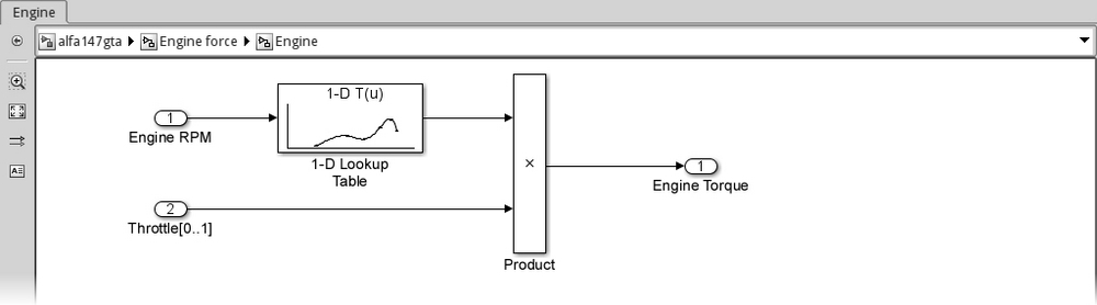
Now that we have the engine RPM, we can model the Engine subsystem.
This subsystem will calculate the engine torque response τEngine. The inputs are the engine RPM coming from the previous subsystem, and the throttle command from the cruise control system. The formula is very simple:
In order to obtain the maximum torque τMAX available at a certain RPM, we need an interpolating block using the following coordinates (taken from the torque curve we saw earlier in this chapter):
|
RPM |
1000 |
1500 |
2000 |
2500 |
3000 |
3500 |
4000 |
4500 |
5000 |
5500 |
6000 |
6500 |
7000 |
|
τMAX |
200 |
220 |
242 |
258 |
260 |
261 |
268 |
285 |
300 |
296 |
290 |
250 |
220 |
Let's add these vectors to the workspace:
EngineRPM = [1000 1500 2000 2500 3000 3500 4000 4500 5000 5500 6000 6500 7000];
EngineTRQ = [200 220 242 258 260 261 268 285 300 296 290 250 220];
We'll place into the Engine subsystem a 1-D Lookup Table (from Simulink | Lookup Tables), double-click on it, and configure it as follows:
- Table dimensions:
1(for each RPM value, we only need one torque value) - Table data:
EngineTRQ(the ordinates) - Breakpoints 1:
EngineRPM(the abscissas) - Interpolation method (in Algorithm tab): Cubic spline (how to calculate the curve between two known points)
- Extrapolation method (in Algorithm tab): Linear (how to calculate the curve outside the RPM range)
The Engine subsystem implementation will look like the following screenshot:
Easy, wasn't it? Now that we have the resulting τEngine we can calculate the force that the engine is applying to the vehicle in the next subsystem.
This subsystem converts the provided engine torque τEngine to the force F applied to the vehicle.
Thanks to Newton's third law, we know that the same force F is applied by the wheels on the ground. Remembering the definition of torque, we can relate F to the wheel torque τWheel and the latter to the engine torque by applying the gear and differential ratios:
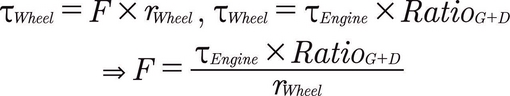
The Simulink implementation of the preceding formula is easily done with the now familiar Product, Divide, and Constant (set to WheelRadius) blocks, like in the following screenshot:
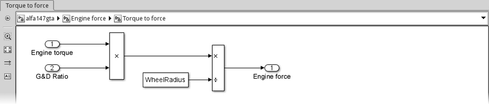
As always, don't forget to update the relevant connections in the parent subsystems.
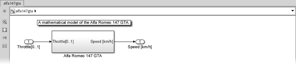
First of all, let's group all the root-level subsystems into one subsystem called Alfa Romeo 147 GTA, and save the current workspace as alfa147gta.mat since we've declared every constant we need.
Then we'll check if we did everything right by running a Simulation | Update Diagram (Ctrl + D). The resulting root subsystem should look like the following screenshot:
That's it! We managed to create a fully usable, fairly accurate car model! Well, we can't steer, but we can surely have drag races!