
Electrical tests to analyse the transport properties of concrete – I: modelling diffusion and electromigration
Abstract
In this chapter, a measurement of electromigration is analysed. The ‘rapid chloride permeability test’ (RCPT) is described in ASTM standard C1202. The aim of the analysis is to obtain the fundamental properties of the concrete (diffusion coefficient and capacity factor) from the test. A computer model is described. The model represents the key processes of diffusion and electromigration using standard equations but then maintains charge neutrality by modelling changes to the voltage distribution. Results are presented to show that the measurement of the non-linearity of the voltage distribution can be used to detect cement replacements such as pulverised fuel ash (PFA) and ground granulated blast furnace slag (GGBS) in concrete.
Key words
rapid chloride permeability test (RCPT); rapid chloride; ASTM C1202; ion–ion interactions; Kirchoff’s law
10.1 Introduction
The ASTM C1202 ‘rapid chloride permeability test’ (RCPT) (ASTM, 2012) is used extensively in many countries to measure the potential durability of concrete structures. However, it emerges that this test is highly complex because several different types of ions are moving and they interact. This is the first of three chapters describing the analysis of this and related tests, and their relevance to durability assessment is discussed in Chapter 13. The fundamental problem that emerges is that the current which is measured in the test is not primarily carried by chloride ions. The main charge carriers are hydroxyl, sodium and potassium ions and the concentrations of these (and thus the current) can be substantially reduced by the addition of pozzolans such as silica fume. Methods to overcome this problem are presented in subsequent chapters.
In this chapter, the processes which occur are described initially at a macroscopic level and then at a microscopic level. Equations are developed to represent the processes, but these cannot be used to give a full solution.
The methods described in Chapter 2 are therefore used to develop a computer model. The model represents the key processes of diffusion and electromigration using standard equations but then maintains charge neutrality by modelling changes to the voltage distribution. This method enables the model to predict current–time transients similar to those recorded in experiments and it can then be used to obtain basic parameters such as diffusion coefficients for tested samples by optimising to the observed data.
Experimental data showing a non-linear voltage distribution is presented together with model results which show that the non-linearity has a significant effect on the current. Other predictions from the model are compared with published data and shown to give good agreement.
10.2 The ASTM C1202 test and the salt bridge
The RCPT was developed by Whiting (1981) and has been standardised as ASTM C1202-12 (ASTM, 2012). The apparatus is shown in Figs 10.1 and 10.2. A steady external electrical potential of 60 V DC is applied to a sample of concrete 50 mm thick and 100 mm diameter for 6 h and the total charge passing is measured as the integral of the current–time transient. The anode and cathode are filled with 0.30 N sodium hydroxide and 3.0 % sodium chloride solutions, respectively. The samples are prepared for the test by vacuum saturation.
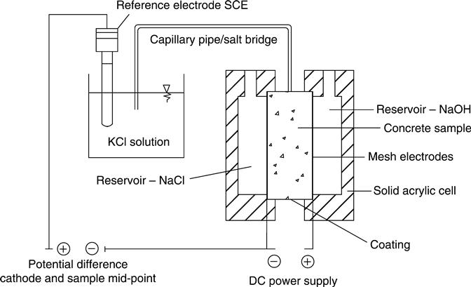
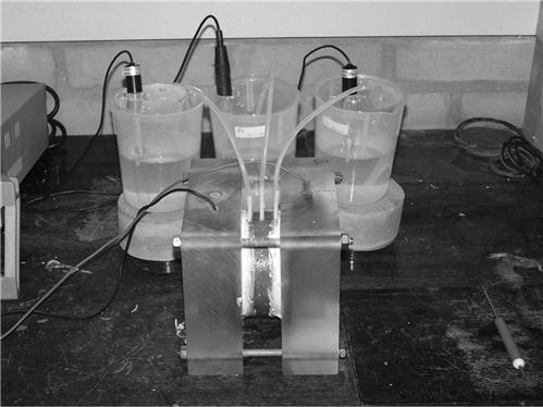
In the work presented here, in addition to the standard test, a salt bridge was added in the middle of the sample to check the voltage distribution (Figs 10.1 and 10.2). A hole of 4 mm diameter and 5–8 mm deep was drilled at the mid-point. The salt bridge used was a solution of 0.1 M potassium chloride which was found to avoid any junction potential at the interface of the salt solution and the pore solution because both ions in it have similar mobility. The salt bridge pipes were 4.5 mm diameter. and were inserted into the hole. The voltage was measured using a saturated calomel electrode (SCE) relative to the cathode cell. The current through the concrete and the voltage at the mid-point were measured continuously every 10 s with a data logger. The membrane potential was calculated by subtracting the value of the voltage measured from the initial value measured at the start of the test.
In previous research, Zhang and Buenfeld (1997) measured the membrane potential across Portland cement (PC) mortar specimens during a diffusion test using reference electrodes and salt bridges in external cells. They found that for different simulated pore solutions, the total junction potentials formed between the measurement devices and the simulated pore solution were in the range of −0.8 and −6 mV. Those values were relatively low compared with the membrane potential measured during the migration tests; therefore, the liquid junction potential formed between the salt bridge and the pore solution concrete sample was not included in the calculations reported here.
The tests were carried out in a temperature controlled room at 21 ± 2 °C. During the tests the temperature was measured continuously in the anodic reservoir. A 3 A, 70 V programmable DC power supply was used although, as noted below, it was often necessary to deviate from the standard and run at voltages below 60 V to avoid over-heating.
The data logger had 16 analogue inputs with 12-bit resolution. A very high input impedance was required in order to ensure that the measuring process did not change the voltage readings. The internal resistance of the data logger had to be significantly greater than the resistance of the concrete during the test, because when measuring voltages the resistance of the equipment itself has an effect on the voltage of the circuit. To achieve the required analogue input performance of the data logger, it had a high resistance voltage divider followed by an operational amplifier configured as a voltage follower.
10.3 The physical processes
10.3.1 The transport processes
The significant transport processes which take place during the test are diffusion and electromigration. These are discussed in Chapter 1. The combined effect of the two processes is given by the Nernst–Planck equation (1.26). Analytical solutions to this equation are available and they are given in Section 10.4. However, they assume that the chloride ion is the only charged particle in the system. The effect of interaction with other ions may be considered on a macroscopic or a microscopic level, and these are discussed in Sections 10.3.2–10.3.3.
10.3.2 Kirchoff’s law
Macroscopically, the procedure to maintain the charge balance is, according to Kirchoff’ s law: ‘… the current density (i) into any point will equal the current out of if’. If the sample is considered (as in a numerical model) as a sequence of cells, this means that for any time the total current in cell i is equal to the current in cell i + 1 (equation 10.1):
[10.1]
The effect of Fick’s law is shown in Fig. 10.3. When a chloride ion enters the sample it cannot just stop because this would violate the law. Something must carry the charge away.
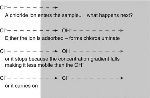
In a diffusion or migration test, the charge build-up generated by differences of mobility of ions in the pore solution is dissipated by the distortion of the electrical field. Only a multi-species system can be physically possible because, if there is only one ion, charge neutrality is never reached.
10.3.3 Ion–ion interactions
The flux F in equation (1.26) has a term in it for the electric field E = dφ/dx. This will arise both from the applied voltage and the distribution of charged ions in the sample.
The field caused by the applied voltage will be uniform across the sample. At the start of the experiment, all of the ions will be in pairs with no net charge but as soon as, for example, a chloride ion migrates into the sample without its sodium pair it will create a field E which will cause a potential difference given by equation (10.2)
[10.2]
This will distort the uniform voltage drop caused by the applied potential. The effect of the field will be to inhibit further migration of ions causing any more build-up of charge. In this way, Kirchoff’s law will take effect and the current into any point within the sample will equal the current out of it. In the solutions at either end of the sample, neutrality will be maintained by ion generation and removal at the electrodes.
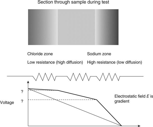
The change in voltage will be a direct effect of different ionic concentrations in the sample. Soon after the start of the test, there will be chloride ions in one side of the sample and sodium in the other side. The regions with these ions in them will have different resistivities due to the different mobilities of the different ions; thus the system is equivalent to three different resistances in series. The voltage drop will depend on the size of each resistance and will not be uniform across the sample. This is shown schematically in Fig. 10.4.
At the start of the test there is assumed to be virtually no chloride in the sample. When the voltage is applied, the chloride ions will start moving into it. If they are to be responsible for the measured current they will be moving without the sodium anions. The rate at which they can flow in will be determined by the number of charge carriers (primarily hydroxyl ions) already available in the sample to carry the current forward to the anode. This concentration of existing charge carriers may be measured as the resistivity of the sample as discussed above. Clearly, if there are no existing charge carriers in the sample (i.e. it is an insulator) no current will flow and chloride will only penetrate by diffusion.
In order to calculate what happens next, it is necessary to consider the physical situation in the sample. Charged ions can only move if charge neutrality is preserved. Thus, for example, a negative chloride ion can only move to a region of the sample if either its sodium counter-ion moves with it or a different negative ion such as a hydroxyl ion is displaced ahead of it. If charge neutrality is not preserved, electric fields build up to prevent the movement. Thus the ability of the chloride ion to move through the region of the sample is determined by the concentration and mobility of other ions in the region. Referring to the Nernst–Einstein equation (1.25), this may be represented as a change in conductivity (or resistivity) of the region. One effect of this is shown in Fig. 10.4. The different resistivities in different regions of the sample make the voltage drop across it non-linear. The difference between the measured voltages and the linear change is known as the membrane potential.
Yu et al. (1993) have carried out experimental measurements of ionic diffusion at an interface between chloride-free and chloride-containing cementitious materials. They observed that the chloride ions obeyed Fick’s law, but the hydroxyl ions distributed themselves to preserve charge balance. This movement would have been caused by an electric field established by the chloride ions and is the mechanism proposed in the present work.
10.3.4 Microscopic considerations
Whenever different ions with different mobilities at different concentrations in the concrete pore solution start to move, there is a tendency for the segregation of charge and the breakdown of the law of electro-neutrality. As a result, several complex and not completely well understood interactions happen in the pore solution, such as the interaction of ions with the solvent or the electrical ion–ion interactions. In order to quantify ion–ion interactions, an electrochemical theory was proposed by Debye and Hückel (1923).
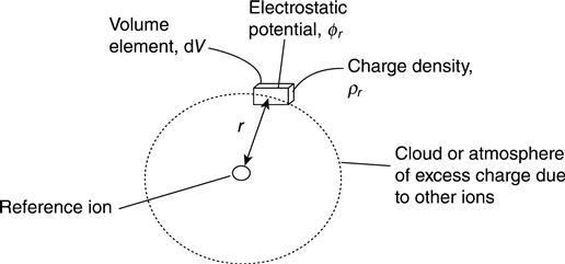
From a ‘simplistic’ microscopic point of view, the Debye and Hückel (ion-cloud) theory can be used to calculate the electrostatic potential contributed by the surrounding ions to the total electric potential at one reference ion. Once a reference ion is selected, the solvent molecules are replaced by a dielectric continuum medium with permittivity ε and the other ions involved are replaced by an excess of charge density (Fig. 10.5). Assuming that the excess charge distribution is spherically symmetrical around the reference ion, the relationship between excess charge density ρr and electrostatic potential φr at a specific radial distance r can be given through Poisson’s equation (10.3) (Bockris and Reddy, 1998):
[10.3]
The excess charge density in the volume element dV is obtained in the Debye–Hückel theory through the linearisation of the Boltzmann equation (equation 10.4):
[10.4]
where:
zi is the valence of ion i
e0 is the electronic charge
ni is the total number of ions i per unit volume
KB is the Boltzmann constant
T is the temperature (K) and
the ∑ symbol refers to all the species i.
Similarly, the maximum value of charge in a spherical cloud is given through the Debye–Hückel length κ−1, which gives an indication of the thickness of the ionic atmosphere from equation (10.5):
[10.5]
The problem can be simplified and linearised and a general equation can be obtained (equation 10.6):
[10.6]
the solution of which is shown as equation (10.7):
[10.7]
It can be seen from equation (10.7) that the microscopic treatment of the electrostatic potential for the ion–ion interaction is highly complex. Further discussion is given by Luping et al. (2012). It has been defined for the reference ion; however, it needs to be applied to the whole concrete system.
Going from a micro to a macro approach, a general model with a larger scale allows a similar, but simpler solution. The simple treatment of the concrete as a circuit in which physical laws must be valid seems to be more appropriate. In that way, the macroscopic electrical model introduced in this chapter permits the inclusion of the ion–ion effects coupling all the species involved to the charge neutrality. This is well suited to analysis with a computer model which is discussed in Section 10.5.
10.4 Analytical solutions
10.4.1 An analytical solution for a single ion
Luping and Nilsson (1992) presented an integrated solution to the Nernst–Planck equation (1.26) which gives the concentration of chloride ions at different times:
[10.8]
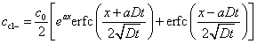 [10.8]
where:
and c0 is the concentration at the surface (in the reservoir).
This may be differentiated to give the current:
[10.9]
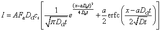 [10.9]
This solution is accurate for a single ion. However, it contains a term for E, the electric field, and the only value that can be used is that for the applied electric field in the tests. It has been shown above (see Fig. 10.4) that E is not a constant across the sample.
10.4.2 Considering multiple ions
If a constant electric potential is applied, as in the ASTM C1202 test, the total flux Ji for each species in the system must be the sum of the migration flux (JM)i and the diffusion flux (JD)i.
[10.10]
Using this notation, equation (1.13) becomes:
[10.11]
where:
Ji is the flux of species i (mol/m2/s)
Di is the diffusion coefficient of species i (m2/s)
ci is the ionic concentration of species i in the pore fluid (mol/m3) and x is the distance (m).
and the Nernst–Planck equation (1.26) becomes:
[10.12]
If used in this form with E as the applied field, the Nernst–Planck equation supposes that the flux of each ion is independent of every other one; however, due to ion–ion interactions, there are ionic fields that affect the final flux. The drift of a species i is affected by the flows of other species present. The law of electroneutrality ensures that no excess of charge is introduced. Under a concrete migration test, the current density into any point will equal the current out of it (Kirchoff’s law):
[10.13]
Faraday’s law states the equivalence of the current density ii and the ionic flux:
[10.14]
In an electrolyte solution in which concentration gradients of the ionic species and an electrical field are present, the total current density (iT) is equal to the sum of the current density produced by the diffusion and the migration conditions:
[10.15]
The total current can be given from equation (10.12):
[10.16]
where ui is the mobility of species i in the pore fluid (m2 s−1 V−1).
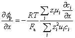
The electric potential gradient is given by two terms: a linear or ohmic potential and a non-linear or membrane potential as in the Nernst–Planck equation:
[10.17]
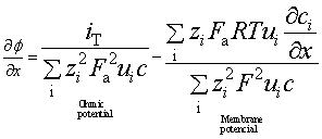 [10.17]
The first term is related to the ohmic potential when an external voltage is applied and gives the charge transfer driven entirely by forces arising from that external voltage. The second term of equation (10.17) is that for the membrane potential gradient δϕp/δx, formed when various charged species have different mobility. In a concrete migration test, the non-linearity of the electric field is due to the membrane potential gradient and it is equivalent to the liquid junction potential (Lorente et al., 2007):
[10.18]
 [10.18]
The overall conductivity of concrete σ can be related to the partial conductivity of one species σi:
[10.19]
where ti is the transference number of species i, which is defined as:
[10.20]
where Qi is the charge contribution of species i and
Q is the total charge passed through the sample.
Thus the electric field due to the diffusion potential can be expressed in terms of the transference number:
[10.21]
10.5 The computer model
10.5.1 Key concepts
The model is similar to the one described in Chapter 2 except that it considers diffusion and electromigration rather than diffusion and advection. It works by repeated application of equations (1.13) and (1.20) through time and space.
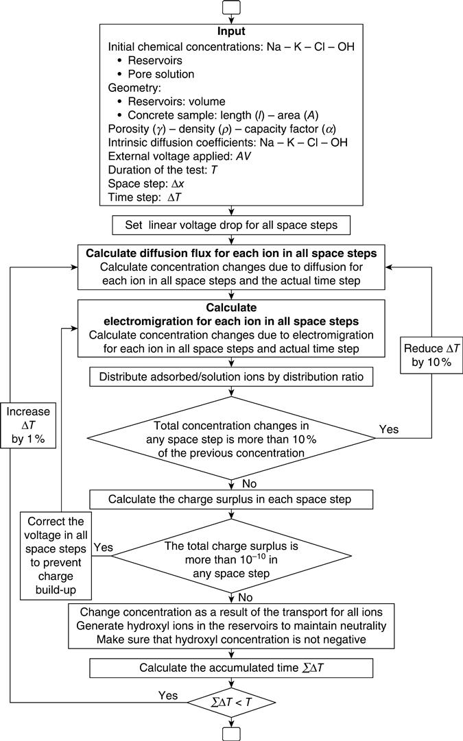
However, in order to apply equation (1.20) it is necessary to know the electric fields. This changes and is extremely difficult to calculate (as shown in Section 10.4). The model therefore avoids this calculation by applying Kirchoff’s law which states that the current must be the same at all points through the sample, i.e. charge neutrality must be maintained. In the computer code, the net charge is calculated for different values of electric field on an iterative basis until the correct value is obtained to achieve neutrality at each time step. The diffusion is calculated initially from equation (1.13). This is unaffected by the electric field. Repeated calculations of electromigration are then made to achieve charge neutrality. By using a process of back-calculation, this is normally achieved in just two or three iterations. This process is shown schematically in Fig. 10.6.

Voltage changes are thus applied within the model by distorting the voltage and checked by ensuring that charge neutrality is maintained throughout the sample at all times. This is clearly not possible if only one ion type is being considered and therefore all of the migrating ions are considered together. The initial concentrations in the sample must be equal for anions and cations and, if the data does not comply with this requirement, the model will not run.
Ion generation and removal at the electrodes is represented in the model by assuming that the ions being generated and removed are always hydroxyl ions. This assumption is probably most accurate at the cathode where hydroxyl ions are produced together with some hydrogen gas. At the anode, hydroxyl ions are removed and the resulting oxygen may be used in corrosion of the electrode, but checks on the sensitivity of the model have shown that this will not cause a significant error.
The sizes of the steps of time and space are set by continuously reducing them and checking that the calculated solution remains constant. In particular, the time step is reduced sufficiently to ensure that the concentration does not change by more than 10 % during any time step. In order to reduce the time required for calculation, the programme progressively increases the time step but, in the early stages of a run, they are kept small by this requirement for stability. The calculations are carried out for ions in solution and at the end of each time step they are redistributed between those adsorbed and those in solution using the capacity factor to calculate adsorption.
The model was proposed for four ions in the pore solution, but can be easily changed to any number of ions. The ions considered were potassium found in the initial pore solution of the sample, sodium and hydroxide found in the pore solution and in the external cells, and chloride found in the external cells.
The transport processes into the concrete were restricted by binding with linear isotherms. A linear isotherm defines a linear relationship between free and the bound ions over a range of concentration at a given temperature, as described in Section 1.3.1. It would be relatively simple to include non-linear binding if data was available to define it. A conceptual diagram of the model is shown in Fig. 10.7.
10.5.2 Temperature
When the current flows, it will cause ohmic heating in the sample. This is regularly observed during the experiments. The heat will be lost at a rate which is approximately proportional to the temperature difference between the sample and room temperature. This effect has been included in the code with a constant of proportionality for the heat loss which was determined from experimental observations of the peak temperatures.
10.5.3 Initial checks
The model was checked against equation (10.9), but this was only possible after disabling the voltage correction, temperature change routines and changes to the concentrations in the reservoirs which are not included in the analytical solution. With these precautions, exact agreement was obtained.
10.6 Initial experimental validation
10.6.1 Methods used in the initial validation
The model described in Section 10.5 will calculate currents and concentrations at different times working from the properties of the ions: diffusion coefficients, capacity factors and initial concentrations. However, the main use of the model is to calculate these properties from results of the experiment, particularly the current–time transient. For this initial work, a simple linear optimisation system was used. In this method, different values for the properties were modelled and the results optimised to fit with the intial current, final current and total charge. The use of artificial neural networks, which is a far more powerful method, is presented in Chapter 11.
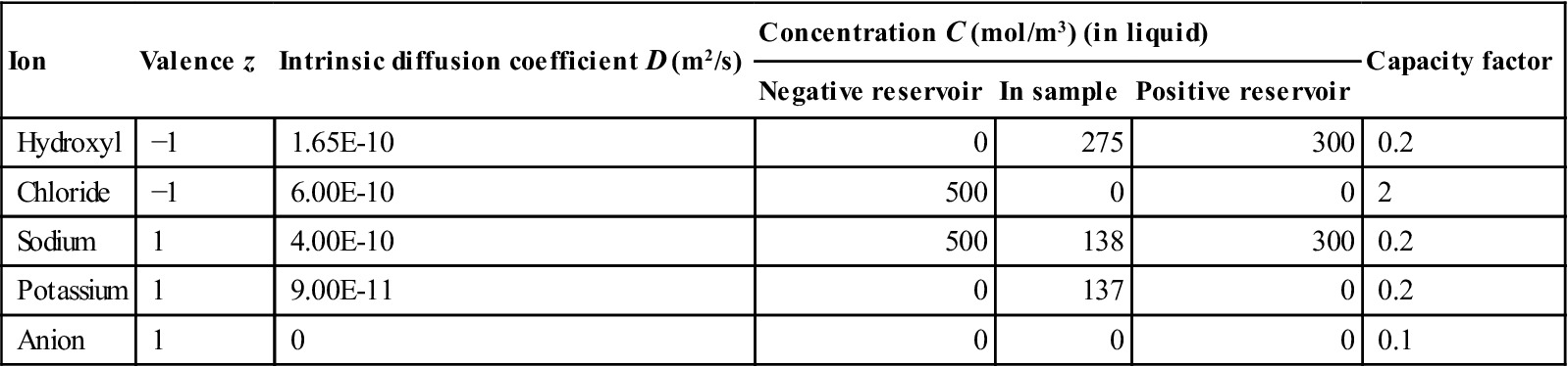
The migration of four ions was considered: chloride, hydroxyl, sodium and potassium. Each of these is defined by three variables: a diffusion coefficient, a capacity factor and an initial concentration in the sample. The programme which was used was capable of optimising three of the resulting 12 variables which define the system. In effect, nine variables had to be set and the remaining three are calculated. The hydroxyl and chloride diffusion and initial concentration of hydroxyl ions were calculated. Table 10.1 shows the initial values of the variables.
Table 10.1
Values for variables at start of run in base case prior to optimisation to fit experimental data
| Ion | Valence z | Intrinsic diffusion coefficient D (m2/s) | Concentration C (mol/m3) (in liquid) | Capacity factor | ||
| Negative reservoir | In sample | Positive reservoir | ||||
| Hydroxyl | −1 | 1.65E-10 | 0 | 275 | 300 | 0.2 |
| Chloride | −1 | 6.00E-10 | 500 | 0 | 0 | 2 |
| Sodium | 1 | 4.00E-10 | 500 | 138 | 300 | 0.2 |
| Potassium | 1 | 9.00E-11 | 0 | 137 | 0 | 0.2 |
| Anion | 1 | 0 | 0 | 0 | 0 | 0.1 |
10.6.2 Mix designs
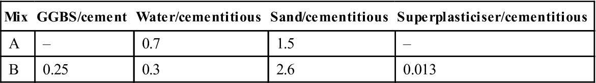
Mixes were cast to the proportions shown in Table 10.2 and cured in water for 28 days. The initial testing was carried out using apparatus which was similar to that described in Section 10.2 but with the following specific differences:
1. The end-volumes were larger at 0.8 l, compared with typical volumes of 0.2 l for the standard apparatus.
2. The experiment was run at 40 V.
3. The samples were run for 1000 min (17 h). These longer runs typically give far greater changes in current during the test than are normally observed during a 6 h test.
4. The cells were designed to give access to the top of the sample. For some samples, this was used to establish a salt bridge by drilling 4 mm diameter holes in the samples and installing a flexible plastic pipe containing 0.1 M potassium chloride. The other end of the pipe was placed in a beaker with a reference electrode.
Table 10.2
Mixes used for experimental work
| Mix | GGBS/cement | Water/cementitious | Sand/cementitious | Superplasticiser/cementitious |
| A | – | 0.7 | 1.5 | – |
| B | 0.25 | 0.3 | 2.6 | 0.013 |
These non-standard cells were developed for this initial work because it was thought that they would be easier to use. However, it was decided for subsequent work that the cells described in the standard (with the addition of the salt bridge) would be used, and this is recommended for any future work.
10.6.3 Fitting the data
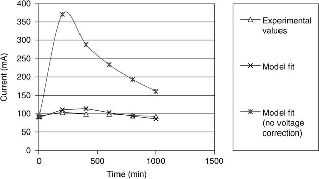
It was observed that optimising with three variables normally gave the model sufficient degrees of freedom to calculate a good theoretical fit to experimental data sets. Figure 10.8 shows the model fit to the data for mix A. This was obtained by optimising to the experimental results. The obtained intrinsic diffusion coefficients were 7.8 × 10⁻¹¹ for hydroxyl and 2.9 × 10⁻¹⁰ for chloride, and the initial concentration of hydroxyl ions was 245 mol/m3. It may be seen that the model was able to give a good fit to the shape of the curve. Figure 10.8 also shows the effect of modelling the system with a linear voltage drop (i.e. no voltage correction), and it may be seen that the effect is significant.
10.6.4 Effect of hydroxyl ion concentration
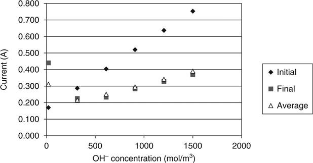
Figure 10.9 shows the predicted effect of the hydroxyl ion concentration on the initial, final and average results. Typically, this concentration would be most affected by the addition of pozzolanic materials which would deplete the free lime during hydration. Sugiyama et al. (2001) observed that the initial current is far more significantly affected by this concentration than the final current, and it may be seen that this observation is well predicted by the model.
10.6.5 Chloride profiles
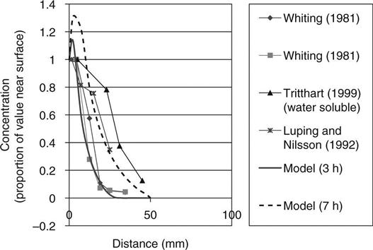
Figure 10.10 shows chloride concentrations predicted by the model at different times and compares them with those found experimentally by different authors. For this modelling, the volume of the input reservoir was increased to reduce predicted changes in concentration. It may be seen that the model predicts a small build-up of chlorides just below the surface that has not been observed, but the shape of the main part of the curve follows the observations.
10.6.6 Salt-bridge measurements
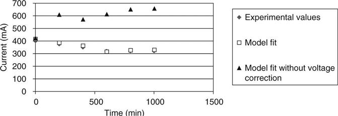
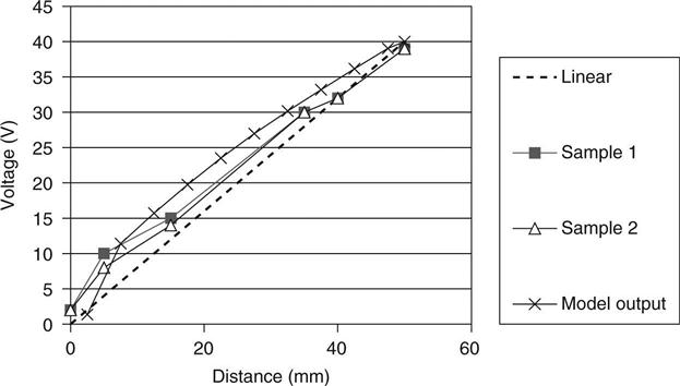
Figure 10.11 shows the current–time transient for a sample of mix B. The fit to this curve was obtained with intrinsic diffusion coefficients of 1.65 × 10⁻¹¹ for hydroxyl and 4 × 10⁻¹¹ for chloride, and the initial concentration of hydroxyl ions was 90 mol/m3. Figure 10.12 shows the voltage distribution across the sample after 6 h indicating the predicted values and two measurements made on replicate samples. It may be seen that the deviation from a linear voltage drop is small, but reference to Fig. 10.11 shows that it has a very significant effect on the current.
10.6.7 Effect of sample length
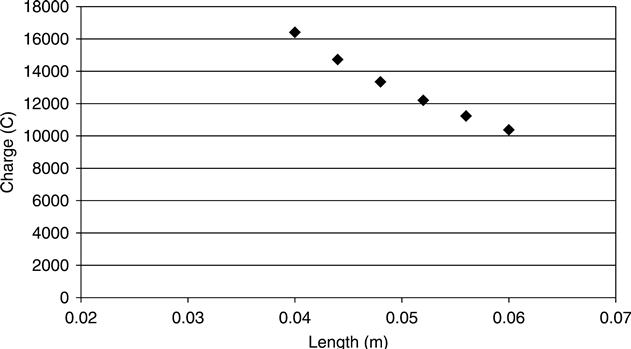
Figure 10.13 shows the predicted effect of changing the sample length. It may be seen that it is non-linear with a greater increase in charge passing at shorter lengths. This effect was observed by Abou-Zeid et al. (2003) for all of a number of series of samples tested.
10.6.8 Discussion
Figures 10.14 and 10.15 show the predicted relationship between the measured charge passing and the diffusion coefficients for chloride and sodium. This basic relationship would be expected, and it has been observed by Yang (2004) and others. Comparing these with Fig. 10.9, it may be seen that it is indicated that a high initial current shows a high hydroxyl concentration, but a high average current (i.e. a current that increases and then falls) shows a high chloride diffusion and a more uniform trend shows high sodium diffusion.
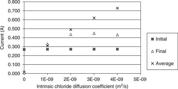
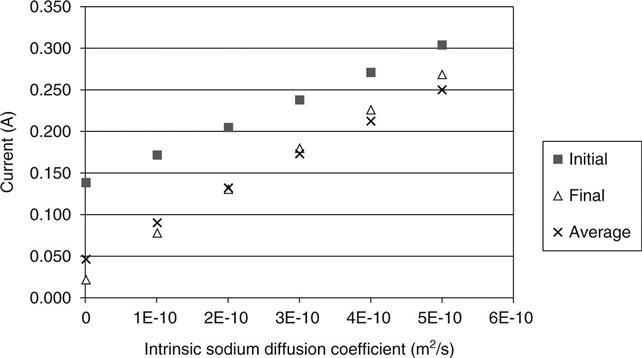
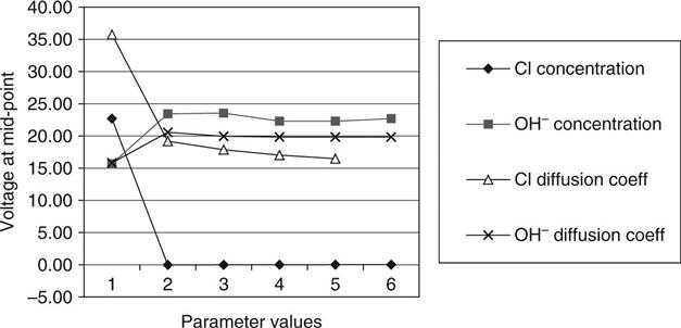
Figure 10.16 shows the predicted voltage at the mid-point of the sample at the end of the test as the different variables are changed. This voltage would be 20 V in a linear voltage distribution (i.e. half the applied voltage). It may be seen that measuring this would yield very useful data for the model to work with and could separate out different phenomena. Pre-saturating the sample with chlorides is predicted to have a very significant effect by reducing the resistivity across all of it except a small region near the anode where the ions are depleted. The hydroxyl ion concentration may be seen to have a significant effect on the mid-point voltage with a change from below 20 V to above 20 V as the concentration increases.
All of the results reported here were taken over a test period of 17 h. It is suggested that this increased time adds significantly to the value of the data. Permitting the reservoir concentrations to change (by limiting their volume) will also cause the current to change more during the test and give a clearer ‘signature’ to show the properties of the sample being tested.
10.7 Full model validation
This work was a far more comprehensive validation of the model carried out in a later programme using ASTM standard cells.
10.7.1 Sample preparation
Mixes of mortar with water to cement (w/c) ratio of 0.49 (mix 1) and 0.65 (mix 2) were cast. Ordinary Portland cement CEM I without mineral or chemical admixtures was used. The binder/sand ratio was 2.75 for all mixes. For each mix, five cylinders of 100 mm diameter and 200 mm height were made to be used both in the porosity and electromigration tests.
The specimens were cured under controlled humidity and temperature, and all the migration tests were made at ages between 28 and 38 days. The cylinders were cut to make samples 50 mm thick and 100 mm diameter. Two samples were taken of each cylinder, being taken from its central part. The test was run on two replicate samples and the reported result is the average of both results.
10.7.2 Porosity measurement
The open porosity accessible by water ε was measured using the simple method of water displacement. The central part of each cylinder (30 mm thickness) was vacuum saturated until constant weight and weighed in water and air. They were then dried in an oven at 105 °C until constant weight and weighed again. The porosity was found with equation (7.9). Three replicates were tested for each mix.
10.7.3 Strength measurement
Three 50 mm cubes for each mix were cast in order to measure the mortar strength. Concrete strengths were obtained from 100 mm cubes.
10.7.4 Electromigration test procedure
Standard cells were used as shown in Fig. 10.2. The anode and cathode reservoir cells were filled with a 0.30 N NaOH and a 3.0 % NaCl solution, respectively (as specified in ASTM C1202), and a DC voltage of 30 V was applied for 21 h. This voltage was lower than that specified in the ASTM standard because 60 V caused unacceptable heating. The current was monitored every 2 min as well as the potential difference between the salt bridges in the sample and the negative electrode of the system.
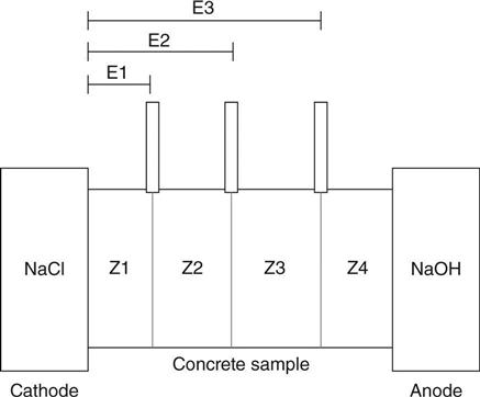
The test was run as described in Section 10.2. For both mixes, the voltages were measured at three different positions. The target location of those points was the mid-point and the quarters of each sample. The distance between the points where the potential was measured and the edge of the sample in contact with the negative electrode (cathode) is shown in Fig. 10.17. The locations of the salt bridges define four zones named as Z1, Z2, Z3 and Z4, and the electric potential difference across each one was measured.
10.7.5 Experimental results
As at the start of the test the electric field is linear across the sample, the gradient or difference between the measured voltage at any time and the linear condition can be calculated. This value corresponds to the membrane potential and was calculated by subtracting the value of the voltage measured from the initial value measured at the start of the test for each time and position:
[10.22]
where:
ΔV corresponds to the membrane potential
VTi is the voltage measured at time t and
V0 is the voltage at the start of the test.
In order to avoid the noise found experimentally during the logging of the tests, a commercial curve fitting software was used. It was found that this noise was substantially reduced by slightly increasing the depths of the drilled holes for the salt bridges. This observation indicates that the noise was caused by the random distribution of aggregate limiting the contact between the salt bridges and the pore volume.
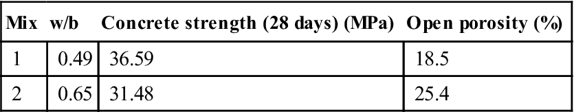
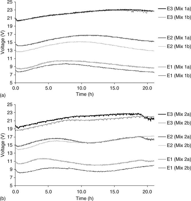
The results of strength and porosity are shown in Table 10.3. Figure 10.18 shows the variation of the voltage across the sample in the mixes tested. Points E1, E2 and E3 are the points where the voltage was measured at the quarters and mid-point of the sample. Although there was noise in the voltage for all the samples, there is a good defined trend and the profile and the replicates in each mix were very similar. The voltage for each sample was not linear with respect to time and position during the test.
Table 10.3
Results of compressive strength and porosity
| Mix | w/b | Concrete strength (28 days) (MPa) | Open porosity (%) |
| 1 | 0.49 | 36.59 | 18.5 |
| 2 | 0.65 | 31.48 | 25.4 |
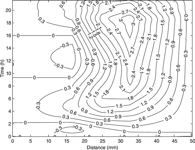
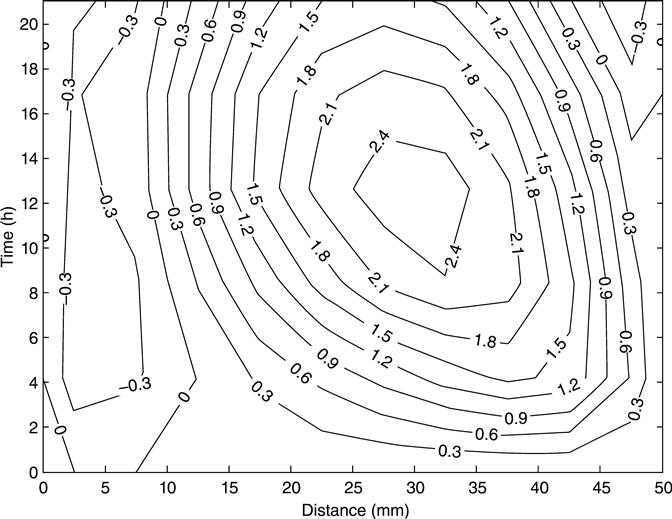
The behaviour of the membrane potential across the samples during the test is shown in Figs 10.19 and 10.20 as contour graphs, each graph represents the average of two samples. The value for the membrane potential at the edges of the sample was assumed as zero because those points correspond to the electrodes in the solutions. Both mixes showed a similar distribution of the membrane potential. There was an increase of voltage in the area that was near to the alkaline solution (positive electrode) and both mixes reached a maximum value of voltage with a subsequent reduction. In the area near to the cathode, the membrane potential either tended to be constant during the test or presented a smooth negative variation.
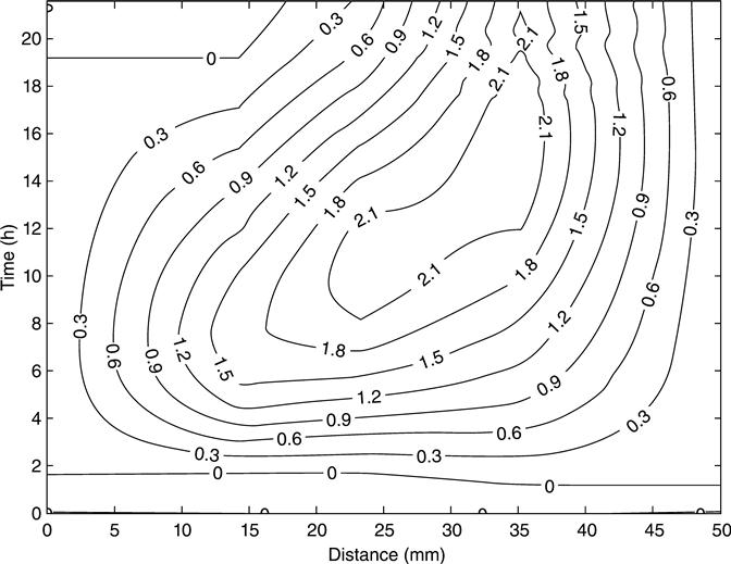
All the membrane potentials at any point throughout the duration of the test can be seen from the contour plots. However, tests of this type are expensive and not easy to complete. As alternative, it has been proposed to study just the behaviour of the mid-point as a source of additional information in a practical situation. It is expected that the mid-point voltage would provide sufficient information for most practical purposes.
10.7.6 Results from the computer model
In order to validate the numerical model, migration tests for both mixes were simulated. The test for mix 1 with water to binder ratio (w/b) = 0.49, was selected as initial comparison and in the simulation of mix 2 (w/b = 0.65) the value of the porosity was adjusted to obtain the value measured experimentally. The characteristics of the system sample/cells are shown in Table 10.4. For this particular simulation, the initial pore solution concentration was based on published results (Bertolini et al., 2013). The intrinsic diffusion coefficients for all the ions were obtained applying an optimisation process for mix 1. The computer program was run enough times to find the best combination of coefficients to fit the experimental values of current and membrane potential in the mid-point of the sample.
Table 10.4
Input parameters at the start of the simulation
| Intrinsic diffusion D (m2/s) | Concentration (mol/m3) upstream (negative) | Concentration (mol/m3) pore solution | Concentration (mol/m3) downstream (positive) | |
| Hydroxyl | 1.60E-10 | 0 | 240 | 300 |
| Chloride | 3.00E-10 | 529 | 0.0 | 0 |
| Sodium | 4.00E-11 | 529 | 79 | 300 |
| Potassium | 9.00E-12 | 0 | 161 | 0 |
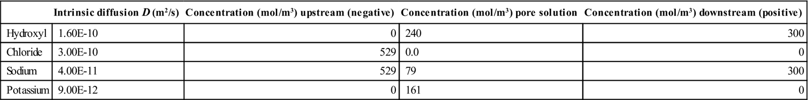
Sample length/radius (m): 0.05/0.05.
Run time (h): 21.
Ext. voltage (V): 30.
Porosity: 0.19.
Cell volume (m3): 0.0002.
Cl capacity factor: 0.3.
The intrinsic diffusion coefficients for sodium and potassium found were significantly lower than the values for chlorides and hydroxides as observed previously by other researchers (Andrade, 1993; Zhang and Buenfeld, 1997). These results confirm that the mobility of cations in porous media differs from that observed if they diffuse in an ideal solution. In the same way, the observed intrinsic diffusion coefficients for chlorides and hydroxides show that both ions are responsible for most transport of charge; however, small changes in the diffusion of cations produce large changes in the mid-point membrane potential. Although the ratio of the intrinsic diffusion coefficients of chloride and hydroxide was greater than 1, it is apparent that the high mobility of chlorides is reduced in the computer model through the adsorption reactions between the ions and the hydration products of concrete which are modelled using a linear isotherm.
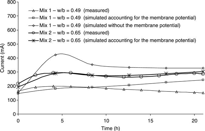
The total electrical current through the samples is shown in Fig. 10.21 where the experimental results are presented with the simulations for mixes one and two. For mix one the current modelled is presented both with the membrane potential and without any voltage correction. The experimental results and the simulation with the membrane potential were in good agreement, being better for initial times than for long times. The difference between them at the end of the tests was around 35 %. In contrast, the profile of the current without including the membrane potential was significantly different to the experimental results. Although the initial current was similar, there was a maximum current value three times greater than when the voltage was corrected. The current passed by mix 2 presented a similar profile for the experimental results and the simulations with the membrane potential corrections. As was expected, mix 2 showed higher values of current because of its higher w/c ratio.
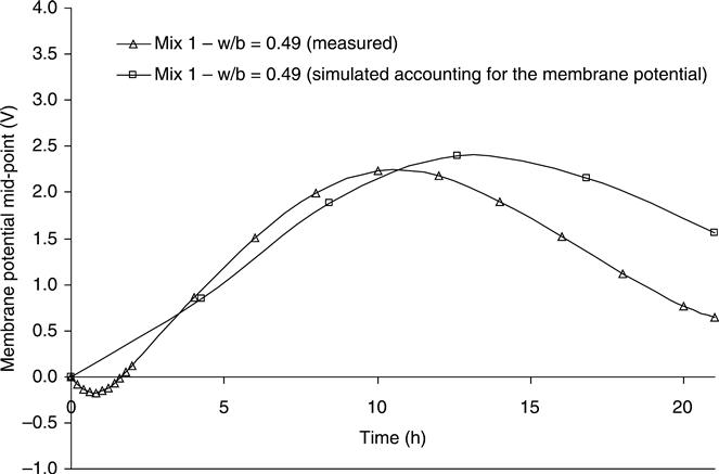
The behaviour of the simulated membrane potential of mix 1 across the sample and during the test is shown in Fig. 10.22 as a contour graph. The numerical values were taken from the numerical program and plotted with the contour function of Matlab®. The simulated membrane potential behaves in the same way as the corresponding experiment (Fig. 10.19). The voltage was negative in the first half of the sample throughout the experiment; in contrast, the second half of the sample had positive values of membrane potential. The simulated and measured mid-point membrane potential is showed in Fig. 10.23 for mix 1. Although the measured profile showed some initial negative values and reached a local maximum membrane potential voltage before the simulations, both graphs showed similar behaviour and have the same profile. From a macroscopic point of view, the local maximum or any feature of the mid-point membrane potential can be explained as a result of the variation of the conductivity of the pore solution due to the migrations of all ions involved. The transient conductivity is defined by the relationship between the transient voltage and the transient current at any point.
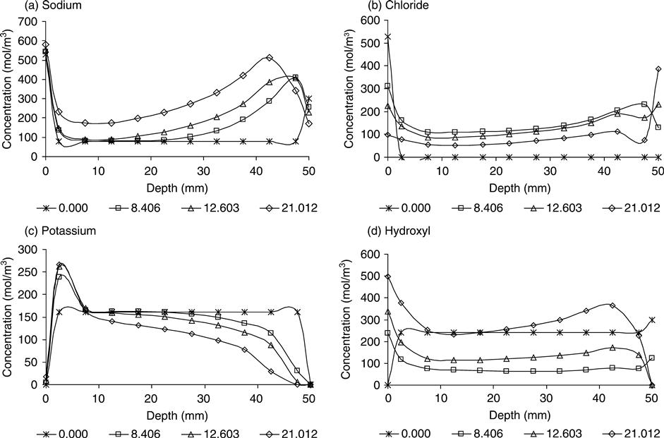
Although the principal aim of the computer model was to simulate the chloride penetration, the profile of the other ions was calculated as result of the interactions between them. The relationship between the transport properties of the chloride and hydroxide ions has been recognised for a long time, however, the transport of potassium and sodium in concrete is not extensively reported in the literature. Figure 10.24 shows the profiles of concentration for the four ions during the simulation of mix 1.
10.7.7 Identifying different mixes
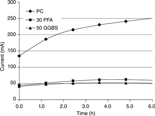
A further use for the measurement of the mid-point potential was identified during this research. Frequently, samples obtained from cores cut from existing structures are tested using the ASTM test and the composition is not known. Figure 10.25 shows the membrane potential at the mid-point voltages from samples containing the most common cement replacement (PFA and GGBS).
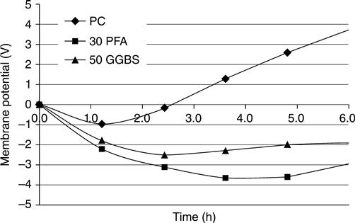
It may be seen from Fig. 10.25 that changing the cementitious components in a mix has a significant effect on ionic voltages. This is because they significantly change the ionic concentrations (e.g. pozzolans deplete hydroxyl ions). These signature traces mean that this test could be used to identify replacement materials.
It may be seen from Fig. 10.26 that the total charge passing is very different for the different mixes. This difference is caused by ion–ion interactions and does not necessarily indicate a change in the diffusion coefficient.
10.8 Conclusions
• It has been proved that the voltage drop in concrete samples during a migration test is not linear with respect to time and position. The application of the Nernst–Planck equation to the simulation of migration of any ionic species through a saturated porous medium accounting for the non-linear voltage allows models to include all the microscopic interactions in a macroscopic way.
• All the ions (sodium, potassium, hydroxide and chlorides) present in a migration test, either in the pore solution or coming from the external cells, need to be included in the simulation in order to account for the non-linear effects caused by differences of mobility. The computer model proposed predicts the transient current and the membrane potential during the experiments.
• If a concrete sample is being tested and it gives a low Coulomb value, this could be caused by a low chloride diffusion coefficient, but it could also be caused by the use of a pozzolanic material to deplete the hydroxyl ions. Measuring the mid-point voltage could differentiate between these two effects and determine whether the sample was as good as the Coulomb value indicated. It is suggested that drilling a small hole and measuring this voltage on a spare channel in the data logger would not add significantly to the cost of these tests but could yield very useful data for analysing the results.