1.1.1 Molecular and ionic transport

The transport processes move materials such as salt or water through concrete. Before considering the processes in detail, the exact nature of what is being transported must be defined. Many molecules will dissociate into two separate parts (ions) when they are in solution with each part carrying an opposite charge. For example common salt (sodium chloride, NaCl) will dissociate into Na⁺ and Cl⁻ and hydrated lime (calcium hydroxide, Ca(OH)₂) will dissociate into Ca⁺⁺ and OH⁻. These ions may move in two different ways. The water itself will move with the ions in it or the ions may move through the water. Thus the transport processes may cause damage both by movement of water (such as pressure-driven flow controlled by permeability) or by ionic movement in the water (such as diffusion or electromigration).

1.1.2 Variability in the properties of the materials

In analytical solutions, it is normally assumed that properties such as permeability, diffusion coefficient and capacity factor remain constant. However, it is well known (Luping et al., 2012) that this is only an approximation. For example, the diffusion coefficient changes with age and the capacity factor with pH (due to carbonation). Including these variations in analytical solutions is difficult and frequently impossible; however, they may be included in numerical solutions if the data is available.

Engineers who normally work with data for the strength of materials will be used to obtaining accurate results from their design calculations and finite element models. The deflection of a structure when loaded in the laboratory or on site will often be within 3 % of that predicted by modelling. This is rarely possible for transport properties. For example, when considering results for permeability testing, Neville (2011) states

The same issues with accuracy apply to diffusion coefficients. While laboratory trials are a necessary first step in work of this kind (in particular for mix design), these results indicate that large site trials are a necessary second step.

1.2.1 Permeability (advection)

Permeability is defined as the property of concrete which measures how fast a fluid will flow through it when pressure is applied. This flow is often referred to as advection (the term permeation is used to refer to a range of different transport processes and can cause confusion). In some types of structure, such as dams and tunnel lining, there may be an external water pressure, but in others it may be capillary suction which creates pressure differentials. The flow is measured as the average speed of the fluid through the solid (the Darcy velocity, V_F).

The volumetric flow is given by:

$F_{\text{v}}=\frac{\text{d}V}{\text{d}t}=A{V}_{\text{F}}{\text{m}}^3/\text{s}$ [1.1]

[1.1]

where:

V is the volume in the reservoir and

A is the cross-section area of flow.

If the flux F is defined as the mass in solution flowing per unit area per second:

$F=C{V}_{\text{F}}\text{kg}/{\text{m}}^2/\text{s}$ [1.2]

[1.2]

where C is the concentration (kg/m³).

The coefficient of permeability k (also known as the hydraulic conductivity) has the units of m/s and is defined from Darcy’s law (Darcy, 1856):

$V_{\text{F}}=\frac{k\left(h_1-h_2\right)}{x}\text{m}/\text{s}$ [1.3]

[1.3]

where the fluid is flowing through a thickness x (m) with pressure heads h₁ and h₂ (m) on each side. The coefficient of permeability is only applicable to water as the permeating fluid and is used in civil engineering because it is used extensively in geotechnology.

The flow rate will depend on the viscosity of the fluid and for this reason the intrinsic permeability is calculated using the viscosity. The intrinsic permeability K has the units of m² and is defined from the equation:

$V_{\text{F}}=\frac{K\left(P_1-P_2\right)}{\text{ex}}\text{m}/\text{s}$ [1.4]

[1.4]

where:

e is the viscosity of the fluid (= 10⁻³ Pa s for water) and

P₁ and P₂ are the pressures on each side (Pa).

The intrinsic permeability is theoretically the same for all different fluids (liquid or gas) permeating through a given porous solid and is thus normally used by scientists.

The pressure from a fluid is given by:

$P=\text{ρgh}$ [1.5]

[1.5]

where:

g = 9.81 m/s² (the gravitational constant)

ρ is the density = 1000 kg/m³ for water and

h is the fluid head (m).

Equating (1.3) and (1.4) thus gives:

$k=\frac{\text{Kρg}}{e}\text{m}/\text{s}$ [1.6]

[1.6]

A typical value of k for water in concrete is 10⁻¹²m/s and thus for K it is 10⁻¹⁹m².

Differential forms of the equations

For analytical solutions the permeability equations should be expressed in differential form:

$V_{\text{F}}=k\frac{\text{d}h}{\text{d}x}=\frac{K}{e}\frac{\text{d}P}{\text{d}x}\text{m}/\text{s}$ [1.7]

[1.7]

Thus:

$F=\frac{\text{KC}}{e}\frac{\text{d}P}{\text{d}x}\text{kg}/{\text{m}}^2/\text{s}$ [1.8]

[1.8]

and, in terms of volumetric flow:

$F_{\text{V}}=\frac{\text{d}V}{\text{d}t}=\frac{\text{KA}}{e}\frac{\text{d}P}{\text{d}x}{\text{m}}^3/\text{s}$ [1.9]

[1.9]

Equations for gas transport

These equations apply to both liquids and gases; however, the analysis of gases is complicated by their compressibility. In order to take account of this, it is necessary to define one ‘mol’ of a material as 6.02 × 10²³ molecules and, from this, the mass of 1 mol of a material with an atomic mass of m is m grams. We now assume that the gas is ‘ideal’ and then the relationship between pressure and volume may be expressed as:

$\text{PV}=\text{nRT}$ [1.10]

[1.10]

where:

n is the number of mols of gas present

R = 8.31 J/mol/K (the gas constant) and

P,V,T are the pressure (Pa), volume (m³) and temperature (K).

Thus, at a given temperature and pressure, one mol of any gas will occupy the same volume.

If the flow is expressed as a change in volume dV/dt, equations (1.9) and (1.10) combine to give the molecular flow rate:

$\frac{\text{d}n}{\text{d}t}=\frac{\text{KAP}}{\text{eRT}}\frac{\text{d}P}{\text{d}x}=\text{JA}\text{mol}/\text{s}$ [1.11]

[1.11]

where:

J is the flux (mol/m²/s) and

A is the area through which the fluid is flowing (m²).

This shows that for a compressible fluid the flow rate will depend on the absolute pressure as well as the pressure gradient.

Knudsen flow at low pressures

The permeability K of a given solid material is assumed to be constant for any fluid with viscosity e transporting through it. However, it has been observed that the permeabilities for liquids and gases are often different. The major reason for the differences between water and gas permeability is the theory of gas slippage. The theory suggests that the permeability will be affected by pressure, which will affect the mean free path of molecules. This gas slippage or ‘Knudsen’ flow becomes significant if the mean free path is of the same order or greater than the size of the capillary through which it is flowing (Knudsen, 1909). The contribution of Knudsen flow to the flow of a given gas is characterised by the Knudsen number, the ratio of the mean free path to the radius of the pores in which the gas is flowing. A Knudsen number significantly greater than unity indicates that Knudsen flow will be important.

Klinkenberg derived an equation relating water and gas permeability to the mean pressure, for oil sands, as follows:

$K_1=\frac{K_{\text{g}}}{\left(1+\frac{b}{P_{\text{m}}}\right)}$ [1.12]

[1.12]

where:

K₁ is the water intrinsic permeability of concrete (m²)

K_g is the gas intrinsic permeability of concrete (m²)

P_m is the mean pressure at which gas is flowing (atmospheres) and

b is a constant known as the Klinkenberg constant.

It may be seen that this indicates that the permeability of a gas will rise significantly at low pressures. Experimental observations of this effect are reported in Chapters 6, 7 and 8.

1.2.2 Diffusion

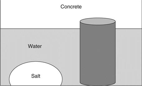
Diffusion is a process by which an ion can pass through saturated concrete without any flow of water. The process is driven by concentration gradient. If a strong solution is in contact with a weak solution they will both tend towards the same concentration. Thus, for example, if a pile of salt is placed in one corner of a container full of water, diffusion will be the process that ensures that when the salt has dissolved it will assume a uniform concentration.

In Fig. 1.1 we intuitively know that as the salt dissolves into the water it will assume an equal concentration at all points throughout the liquid. By the same mechanism, ions which are present in the pore water of the concrete will diffuse out and also assume an equal concentration throughout the liquid. Note that it is assumed that the water does not move.

Moisture diffusion will take place in a gas when the concentration of water vapour is higher in one region than another. This mechanism will enable water to travel through the pores of unsaturated concrete (but may be considered as permeability caused by a vapour pressure – see below in this section). The ions will generally diffuse in pairs with equal and opposite charges. If they do not do this they will build up an electrical potential which will cause them to electromigrate back together (see Section 1.2.3 below).

Diffusion is normally defined in terms of flux F which is the flow per second per unit cross-sectional area of the porous material. Flux may be measured in kg/m²/s although a unit of mol/m²/sec (designated J) is also common. The diffusion coefficient is defined from the equation (1.13) which has been known empirically since 1855 as Fick’s first law (Fick, 1855):

$F=D\frac{\text{d}C}{\text{d}x}\text{kg}/{\text{m}}^2/\text{s}$ [1.13]

[1.13]

where D is the diffusion coefficient (m²/s). This equation also applies if flux is measured in mol/m²/s and concentration in mol/m³.

Considering a small element of the system, the rate at which the concentration changes with time will be proportional to the difference between the flux into it and the flux out of it:

$V\frac{\text{d}C}{\text{d}t}=A\text{Δ}F$ [1.14]

[1.14]

where:

V is the volume of the element

A is the cross-sectional area and

L = V/A is the length.

$\text{Δ}F=L\frac{\text{d}F}{\text{d}x}$ [1.15]

[1.15]

Thus:

$\frac{\text{d}C}{\text{d}t}=\frac{\text{d}F}{\text{d}x}$ [1.16]

[1.16]

and:

$\frac{\text{d}C}{\text{d}t}=D\frac{{\text{d}}^{2}C}{\text{d}{x}^2}$ [1.17]

[1.17]

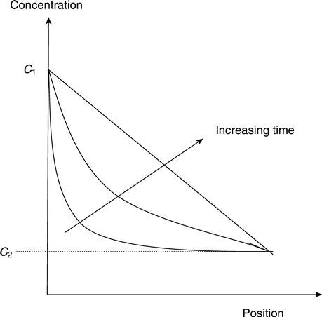
Considering a system with concentrations C₁ and C₂ on each side (see Fig. 1.2), looking first at the long-term solution, the system will eventually reach a state where the concentration stops changing. Thus dC/dt = 0 and therefore dC/dx is constant. Before this happens, the rate of change of concentration with time (dC/dt), and thus the curvature of the concentration vs position curve (d²C/dx²), will progressively decrease. dC/dt will also increase with D, i.e. the system will reach a steady state sooner if the diffusion coefficient is higher (the flux will also be greater).

Comparing diffusion coefficients and permeability

When considering the movement of a gas or vapour which is mixed with another gas (e.g. water vapour in air), it is instructive to compare the equations for permeability and diffusion. Equation (1.10) shows that the concentration is proportional to the pressure.

For a fluid with atomic mass m:

$C=\frac{\text{mn}}{V}$ [1.18]

[1.18]

Substituting this into equations (1.8), (1.10) and (1.13) gives:

$D=\frac{\text{KCRT}}{\text{me}}$ [1.19]

[1.19]

Thus the coefficients for permeability and diffusion are exactly related and this transport may be considered as either diffusion or advection and the equations will give the same answer.

1.2.3 Electromigration

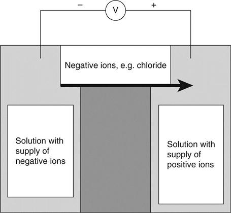
Electromigration (often called migration) occurs when an electric field (voltage difference) is present. This may be derived from an external source such as leakage from a direct current power supply but is also frequently caused by the electrical potential of pitting corrosion on reinforcing steel. If an electric field is applied across the concrete in Fig. 1.3, the negative ions will move towards the positive electrode.

Electromigration can be measured from the electrical resistance of the concrete because it is the only mechanism by which concrete can conduct electricity. The flux due to electromigration is given by equation (1.20):

$F=\frac{DzEC{F}_{\text{a}}}{\text{RT}}\text{kg}/{\text{m}}^2/\text{s}$ [1.20]

[1.20]

where:

z is the valence of the ion (i.e. the charge on it divided by the charge of an electron)

F_a is the Faraday constant = 9.65 × 10⁴C/mol

E is the electric field (V/m)

R = 8.31 J/mol/K and

T is the temperature (K).

The flux can be expressed as an electric current:

$I=zF{F}_{\text{a}}A\text{A}$ [1.21]

[1.21]

Ohm’s law states that:

$R=\frac{ɸ}{I}\text{Ω}$ [1.22]

[1.22]

where ɸ is the voltage. The electric field is the voltage gradient and thus:

$E=\frac{ɸ}{x}=\frac{\text{IR}}{x}=\frac{zF{F}_{\text{a}}AR}{x}\text{V}/\text{m}$ [1.23]

[1.23]

where x is the distance (m). The resistivity ρ is defined from the equation:

$R=\frac{\text{ρx}}{A}=\frac{x}{\text{Aσ}}\text{Ω}$ [1.24]

[1.24]

where σ is the electrical conductivity in (Ωm)⁻¹, the inverse of the resistivity.

Rearranging equations (1.20), (1.23) and (1.24) gives the Nernst–Einstein equation:

$D=\frac{\text{RTσ}}{z^2{F}_{\text{a}}^{2}C}$ [1.25]

[1.25]

Note that if this is to be measured, an alternating current must be used to prevent polarisation. These phenomena are discussed in detail in Chapters 10, 11 and 12.

1.2.4 Combining diffusion and electromigration

The general law governing the ionic movements due to the chemical and electrical potential is obtained by combining equations (1.13) and (1.20) and is known as the Nernst–Planck equation:

$F=D\frac{\partial C}{\partial x}+\frac{z{F}_{\text{a}}}{\text{RT}}DC\frac{\partial ɸ}{\partial x}$ [1.26]

[1.26]

1.2.5 Thermal gradient

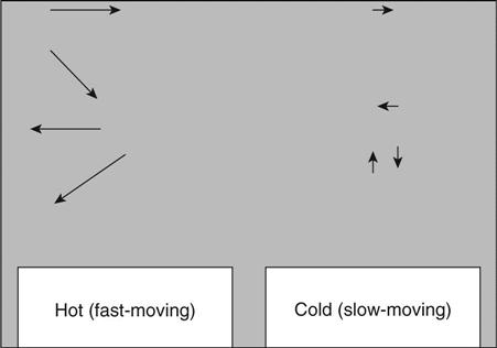
Water will move from hot regions to cold regions in solids. The rate at which it moves will depend on the permeability of the solid. This process is independent of and additional to the drying process (evaporation) which will take place on exposed surfaces which are hot. Similarly, in saturated concrete, ions in hotter water will migrate towards colder regions. The mechanism is shown in Fig. 1.4 and depends on probability. At a microscopic level, the temperature of a solid is a measure of the kinetic energy of the atoms and molecules within it. An ion or molecule which is moving faster on the hot side has a greater probability of crossing the sample than one on the cold side.

The most obvious situation when this process may occur is when a concrete structure which has been contaminated with de-icing salt heats up in sunlight. The salt saturated water in the surface pores will migrate rapidly into the structure. Even if this does not reach the steel by this mechanism, the salt may diffuse the remaining distance.

1.3.1 Adsorption

When considering transport of ions in a porous material, it is essential to consider adsorption at the same time because in many situations the bulk of the ions which enter into a barrier will be adsorbed before they reach the other side. Adsorbed ions are bound into the matrix in various ways and are unable to move and therefore unable to cause any deterioration.

We define:

C₁ kg/m³ is the concentration of ions per unit volume of liquid in the pores (i.e. the mobile ions)

and

C_s kg/m³ is the total concentration (including immobile adsorbed ions) per unit volume of the solid.

It is necessary to make a clear distinction between absorption and adsorption. The term absorption is used to describe processes such as capillary suction and osmosis which may draw water into concrete. Adsorption is the term used for all processes which may bind an ion (temporarily or permanently) in the concrete and prevent it from moving. These processes may be chemical reactions or a range of physical surface effects.

When the ionic concentration in a concrete sample is measured there are various different systems that can be used:

The ratio of the solid to liquid concentrations is known as the capacity factor α. In concrete, the adsorption of chloride ions is normally on the cement (binding on the aluminate phases). Thus the capacity factor will be proportional to the cement content. It will probably also be higher if pulverised fuel ash or GGBS is used.

A simple approximation of the amount of material which is adsorbed onto the matrix may be obtained by assuming that at all concentrations it is proportional to the concentration of ions in the pore fluid (note that this implies that the adsorption is reversible). Thus the capacity factor is a constant for all concentrations. This approximation is useful for modelling, but it works best for low solubility ions, unlike chlorides, which have a solubility of about 10 %. For chlorides, there will still be a good link between the number in solution and the number adsorbed, but it will not be a completely linear relationship. There are many other ways of analysing adsorption, for example the ‘Langmuir isotherm’ gives a more complex relationship between C_s and C₁. These more complex isotherms could be used in computer modelling but are difficult to use in analytical solutions (Luping et al., 2012).

Using the linear isotherm, the ratio of the two concentrations is constant and is the capacity factor:

$\alpha =\frac{C_{\text{s}}}{C_1}$ [1.27]

[1.27]

Equation (1.16) for the rate of change of concentration will be for the total concentration:

$\frac{\text{d}{C}_{\text{s}}}{\text{d}t}=\frac{\text{d}F}{\text{d}x}$ [1.28]

[1.28]

Thus:

$\frac{\text{d}{C}_1}{\text{d}t}=\frac{1}{\alpha }\frac{\text{d}F}{\text{d}x}$ [1.29]

[1.29]

From this, it may be seen that a high value of α will make the concentration change much more slowly – i.e. if chlorides are penetrating into a wall it will delay the start of corrosion of the steel.

1.3.2 Diffusion with adsorption

Because there are two different ways of measuring concentration in an adsorbing system, there are also two different ways of measuring diffusion: (i) using the apparent diffusion coefficient D_a (also known as the ‘effective’ diffusion coefficient; and (ii) using the intrinsic diffusion coefficient D_i.

The apparent diffusion coefficient D_a (which is what can be measured by testing the solid using measurements of total concentration) is defined from measurements of total concentration:

$F=D_{\text{a}}\frac{\text{d}{C}_{\text{s}}}{\text{d}x}\text{kg}/{\text{m}}^2/\text{s}$ [1.30]

[1.30]

The intrinsic diffusion coefficient D_i (which is the diffusion coefficient for the pore solution) is defined from measurements of the water soluble concentration:

$F^{\prime }=D_{\text{i}}\frac{\text{d}{C}_1}{\text{d}x}\text{kg}/{\text{m}}^2/\text{s}$ [1.31]

[1.31]

where F′ is the flux per unit cross-sectional area of the liquid in the pores.

Thus:

$F=\epsilon D_{\text{i}}\frac{\text{d}{C}_1}{\text{d}x}\text{kg}/{\text{m}}^2/\text{s}$ [1.32]

[1.32]

where ε is the porosity.

By integrating these (or by inspection) it may be seen that:

$\frac{\alpha }{\epsilon }=\frac{D_{\text{i}}}{D_{\text{a}}}$ [1.33]

[1.33]

For a typical concrete D_i = 5 × 10⁻¹²m²/s.

1.3.3 Capillary suction

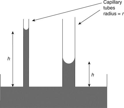
Capillary suction occurs in fine voids (capillaries) with wetting surfaces and is caused by surface tension. In the experiment shown in Fig. 1.5, water rises higher up a smaller diameter glass capillary tube and this shows how this mechanism has greatest effect in systems with fine pores. This leads to the situation that concretes with finer pore structures (normally higher grade concretes) will experience greater capillary suction pressures. Fortunately, the effect is reduced by the restriction of flow by generally lower permeabilities.

A good demonstration of the power of capillary suction in concrete can be observed by placing a cube in a tray of salt water and simply leaving it in a dry room for several months. The water with the salt in it will be drawn up the cube by ‘wicking’ until it is close to an exposed surface and can evaporate. As this happens, the near-surface pores fill up with crystalline salt which will eventually achieve sufficient pressure to cause spalling. This mechanism of damage by salt crystallisation is common in climates where there is little rain to wash the salt out again.

The capillary suction will create a pressure:

$P=\frac{2s}{r}$ [1.34]

[1.34]

where:

s is the surface tension of the water (N/m) (= 0.073 N/m for water) and r is the radius of the pores (m).

Thus, since the pressure from a fluid P = ρ g h, the height of the column of water in a fully wetting capillary is given by:

$h=\frac{2s}{\text{rρg}}\text{m}$ [1.35]

[1.35]

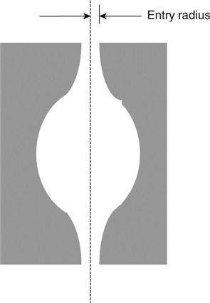
A typical pore in concrete has a radius of 10⁻⁸m. Putting this into the equation gives a height of 1460 m indicating that damp should rise up concrete to this height. The reason why it does not is the irregularity of the pores (see Fig. 1.6). Water will be drawn up through the neck of the pore but will then reach the point where the radius is much larger and the capillary suction pressure thus much lower and will stop at that point.

1.3.4 Osmosis

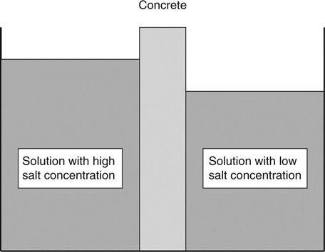
Osmosis depends on what is called a semi-permeable membrane. This is a barrier through which the water can pass but material dissolved in it cannot pass as easily. An example is the surface layer of concrete which will permit water to enter but restrict the movement of the lime dissolved in the pore water. The osmotic effect causes a flow of water from the weak solution to the strong solution. Thus water on the outside of concrete (almost pure, i.e. a weak solution) is drawn into the pores where there is a stronger solution. The process is illustrated in Fig. 1.7. If two solutions were placed either side of a barrier as shown, the level in one of them would rise, although in practice this would be very difficult to observe because concrete is permeable and the liquid would start to flow back as soon as a pressure difference developed.

If different solutions are present on each side of the sample, osmosis will still take place even if the concentrations are the same. The direction of flow will depend on their relative ‘osmotic coefficients’. Osmosis could be a significant process for drawing chlorides and sulphates into concrete. Having entered the concrete they may move further in by diffusion.

1.3.5 Electro-osmosis

If a solid material has an electrically charged surface, the water in the pores will acquire a small opposite charge. Clay, both in soil and bricks, has a negatively charged surface so the pore water will have a positive charge. The water will thus move towards a negatively charged plate and away from a positively charged one. This system is used in one of the commercially available systems for removing damp from existing buildings (the more common one is resin injection to block the pores).