
While diffusion and contagion are not identical, there are certainly some shared elements we can leverage for our analysis prior to jumping into a visual assessment using Gephi. Remember, in our contagion discussion, the importance of physical contact coupled with the probability of transmission as critical elements in spreading the disease. With diffusion, we recognize that physical contact is not necessarily required for spreading information, but there is still a probability element at work, especially when product adoption is involved. I'll illustrate this briefly before we move onto the graphs.
Suppose a new tablet is planned for upcoming release, supported by a large marketing campaign and plenty of insider buzz about the virtues of the product. Some of your friends have talked about getting the new tablet, but you are unsure whether it's worth the investment, as you already have a perfectly capable unit purchased just 12 months earlier. What factors will sway you in one direction (purchase) or the other (don't purchase)? It might well be the behavior of your closest friends who will be the primary influence in your purchase decision. How does all of this relate to contagion? It relates through our use of probability. As with the contagion examples, there are probabilities associated with your decision to purchase or not to purchase. If many of your friends decide to buy the new tablet, it is more likely that you will also make this decision, as your collective probability has increased. In this sense, it is akin to the transmission of an infectious disease, albeit without (perhaps) the physical contact. A higher purchase probability leads to further spread of the new product, and the product sales continue to increase as it spreads further into the market.
Now it's time to see how this process can unfold using some examples from Gephi. As we did with our contagion illustration, we'll walk you through a rather simple example using a random network of 50 nodes; although in this case, we'll increase the connectivity level so that the network consists of a single giant component. Our case will be based on the release of a new cell phone that provides an attractive feature set that will influence some consumers to replace their old phones.
We will make some assumptions about our network:
- Our network will consist of 50 individuals who are all connected to at least one or the other node within the network. We'll again use the Random Graph generator in Gephi to build a simple network to illustrate the diffusion process.
- Each individual in the network will invest in the new phone only if at least one-third of their direct contacts also purchase the phone. For example, a person with four direct contacts, but just one who has purchased the phone, will not be influenced enough to purchase the phone themselves. However, if two or more of his/her friends already have the phone, then he/she will also make the purchase.
Let's begin to examine the diffusion process for this product. We're using the Out-degree measure to define who the primary influencers are within this network and sizing the nodes to reflect this influence. Our initial graph will reflect t0, when a few early adopters have elected to purchase the new phone. These adopters are identified using darker shading, as shown in the following diagram:
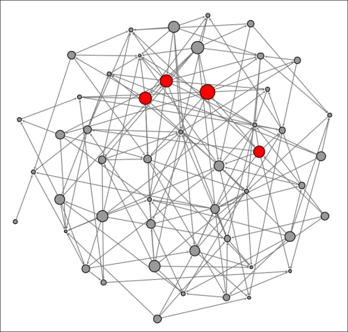
Diffusion network at t0
As alluded to earlier, we see four early adopters who appear to have significant influence levels within the network based on their number of out degrees (as depicted by node size). Just how influential they are remains to be seen as we iterate through time periods. For the sake of this discussion, let's assume that each snapshot represents a weekly interval, as potential buyers need some time to consider their purchase likelihood. For this example, we will show all purchasers in a cumulative manner, as they will be unlikely to consider a new tablet for another year or two.
One week later at t+1 several new purchasers have appeared, as at least one-third of their direct contacts have purchased the phone previously:
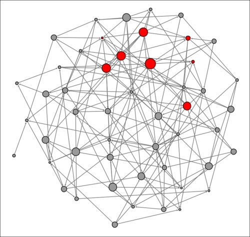
Diffusion network at t+1
Four new buyers have appeared, while others have yet to purchase the phone, opting to wait for a higher proportion of their friends to make a purchase. Now let's take a look at t+2 to see how many incremental buyers have been sufficiently influenced by their friend's purchase decision:
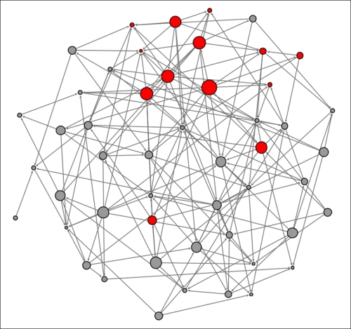
Diffusion network at t+2
Another four people have elected to purchase the new phone based on their friends' behavior, including two buyers with more distant but still direct connections. After just two weeks, nearly 25 percent of the network members have elected to buy this phone; while this might not equate to the diffusion level of a viral video on the Web; it does appear to represent a successful level of product adoption through the diffusion process.
This represents a very basic diffusion example; there are additional factors that can be employed in displaying the diffusion process, many of which can be discovered through resources listed in the Appendix, Data Sources and Other Web Resources. Also, as we mentioned in the discussion on contagion, some more dynamic examples of diffusion will be shared in Chapter 8, Dynamic Networks, which employ datasets with time elements.