
Bayesian inference is a method of learning about the relationship between variables from data, in the presence of uncertainty, in real-world problems. It is one of the frameworks of probability theory. Any reader interested in Bayesian inference should have a good knowledge of probability theory to understand and use Bayesian inference. This chapter covers an overview of probability theory, which will be sufficient to understand the rest of the chapters in this book.
It was Pierre-Simon Laplace who first proposed a formal definition of probability with mathematical rigor. This definition is called the Classical Definition and it states the following:
The theory of chance consists in reducing all the events of the same kind to a certain number of cases equally possible, that is to say, to such as we may be equally undecided about in regard to their existence, and in determining the number of cases favorable to the event whose probability is sought. The ratio of this number to that of all the cases possible is the measure of this probability, which is thus simply a fraction whose numerator is the number of favorable cases and whose denominator is the number of all the cases possible. | ||
| --Pierre-Simon Laplace, A Philosophical Essay on Probabilities | ||
What this definition means is that, if a random experiment can result in ![]() mutually exclusive and equally likely outcomes, the probability of the event
mutually exclusive and equally likely outcomes, the probability of the event ![]() is given by:
is given by:

Here, ![]() is the number of occurrences of the event
is the number of occurrences of the event ![]() .
.
To illustrate this concept, let us take a simple example of a rolling dice. If the dice is a fair dice, then all the faces will have an equal chance of showing up when the dice is rolled. Then, the probability of each face showing up is 1/6. However, when one rolls the dice 100 times, all the faces will not come in equal proportions of 1/6 due to random fluctuations. The estimate of probability of each face is the number of times the face shows up divided by the number of rolls. As the denominator is very large, this ratio will be close to 1/6.
In the long run, this classical definition treats the probability of an uncertain event as the relative frequency of its occurrence. This is also called a frequentist approach to probability. Although this approach is suitable for a large class of problems, there are cases where this type of approach cannot be used. As an example, consider the following question: Is Pataliputra the name of an ancient city or a king? In such cases, we have a degree of belief in various plausible answers, but it is not based on counts in the outcome of an experiment (in the Sanskrit language Putra means son, therefore some people may believe that Pataliputra is the name of an ancient king in India, but it is a city).
Another example is, What is the chance of the Democratic Party winning the election in 2016 in America? Some people may believe it is 1/2 and some people may believe it is 2/3. In this case, probability is defined as the degree of belief of a person in the outcome of an uncertain event. This is called the subjective definition of probability.
One of the limitations of the classical or frequentist definition of probability is that it cannot address subjective probabilities. As we will see later in this book, Bayesian inference is a natural framework for treating both frequentist and subjective interpretations of probability.
In both classical and Bayesian approaches, a probability distribution function is the central quantity, which captures all of the information about the relationship between variables in the presence of uncertainty. A probability distribution assigns a probability value to each measurable subset of outcomes of a random experiment. The variable involved could be discrete or continuous, and univariate or multivariate. Although people use slightly different terminologies, the commonly used probability distributions for the different types of random variables are as follows:
One of the well-known distribution functions is the normal or Gaussian distribution, which is named after Carl Friedrich Gauss, a famous German mathematician and physicist. It is also known by the name bell curve because of its shape. The mathematical form of this distribution is given by:

Here, ![]() is the mean or location parameter and
is the mean or location parameter and ![]() is the standard deviation or scale parameter (
is the standard deviation or scale parameter (![]() is called variance). The following graphs show what the distribution looks like for different values of location and scale parameters:
is called variance). The following graphs show what the distribution looks like for different values of location and scale parameters:

One can see that as the mean changes, the location of the peak of the distribution changes. Similarly, when the standard deviation changes, the width of the distribution also changes.
Many natural datasets follow normal distribution because, according to the central limit theorem, any random variable that can be composed as a mean of independent random variables will have a normal distribution. This is irrespective of the form of the distribution of this random variable, as long as they have finite mean and variance and all are drawn from the same original distribution. A normal distribution is also very popular among data scientists because in many statistical inferences, theoretical results can be derived if the underlying distribution is normal.
Now, let us look at the multidimensional version of normal distribution. If the random variable is an N-dimensional vector, x is denoted by:
Then, the corresponding normal distribution is given by:

Here, ![]() corresponds to the mean (also called location) and
corresponds to the mean (also called location) and ![]() is an N x N covariance matrix (also called scale).
is an N x N covariance matrix (also called scale).
To get a better understanding of the multidimensional normal distribution, let us take the case of two dimensions. In this case, ![]() and the covariance matrix is given by:
and the covariance matrix is given by:

Here, ![]() and
and ![]() are the variances along
are the variances along ![]() and
and ![]() directions, and
directions, and ![]() is the correlation between
is the correlation between ![]() and
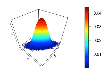
and ![]() . A plot of two-dimensional normal distribution for
. A plot of two-dimensional normal distribution for ![]() ,
, ![]() , and
, and ![]() is shown in the following image:
is shown in the following image:
If ![]() , then the two-dimensional normal distribution will be reduced to the product of two one-dimensional normal distributions, since
, then the two-dimensional normal distribution will be reduced to the product of two one-dimensional normal distributions, since ![]() would become diagonal in this case. The following 2D projections of normal distribution for the same values of
would become diagonal in this case. The following 2D projections of normal distribution for the same values of ![]() and
and ![]() but with
but with ![]() and
and ![]() illustrate this case:
illustrate this case:

The high correlation between x and y in the first case forces most of the data points along the 45 degree line and makes the distribution more anisotropic; whereas, in the second case, when the correlation is zero, the distribution is more isotropic.
We will briefly review some of the other well-known distributions used in Bayesian inference here.