
As the name suggests, artificial neural networks are statistical models built taking inspirations from the architecture and cognitive capabilities of biological brains. Neural network models typically have a layered architecture consisting of a large number of neurons in each layer, and neurons between different layers are connected. The first layer is called input layer, the last layer is called output layer, and the rest of the layers in the middle are called hidden layers. Each neuron has a state that is determined by a nonlinear function of the state of all neurons connected to it. Each connection has a weight that is determined from the training data containing a set of input and output pairs. This kind of layered architecture of neurons and their connections is present in the neocortex region of human brain and is considered to be responsible for higher functions such as sensory perception and language understanding.
The first computational model for neural network was proposed by Warren McCulloch and Walter Pitts in 1943. Around the same time, psychologist Donald Hebb created a hypothesis of learning based on the mechanism of excitation and adaptation of neurons that is known as Hebb's rule. The hypothesis can be summarized by saying Neurons that fire together, wire together. Although there were several researchers who tried to implement computational models of neural networks, it was Frank Rosenblatt in 1958 who first created an algorithm for pattern recognition using a two-layer neural network called Perceptron.
The research and applications of neural networks had both stagnant and great periods of progress during 1970-2010. Some of the landmarks in the history of neural networks are the invention of the backpropagation algorithm by Paul Werbos in 1975, a fast learning algorithm for learning multilayer neural networks (also called deep learning networks) by Geoffrey Hinton in 2006, and the use of GPGPUs to achieve greater computational power required for processing neural networks in the latter half of the last decade.
Today, neural network models and their applications have again taken a central stage in artificial intelligence with applications in computer vision, speech recognition, and natural language understanding. This is the reason this book has devoted one chapter specifically to this subject. The importance of Bayesian inference in neural network models will become clear when we go into detail in later sections.
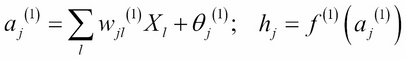
Let us look at the formal definition of a two-layer neural network. We follow the notations and description used by David MacKay (reference 1, 2, and 3 in the References section of this chapter). The input to the NN is given by ![]() . The input values are first multiplied by a set of weights to produce a weighted linear combination and then transformed using a nonlinear function to produce values of the state of neurons in the hidden layer:
. The input values are first multiplied by a set of weights to produce a weighted linear combination and then transformed using a nonlinear function to produce values of the state of neurons in the hidden layer:
A similar operation is done at the second layer to produce final output values ![]() :
:

The function ![]() is usually taken as either a
sigmoid function
is usually taken as either a
sigmoid function ![]() or
or ![]() . Another common function used for multiclass classification is softmax defined as follows:
. Another common function used for multiclass classification is softmax defined as follows:

This is a normalized exponential function.
All these are highly nonlinear functions exhibiting the property that the output value has a sharp increase as a function of the input. This nonlinear property gives neural networks more computational flexibility than standard linear or generalized linear models. Here, ![]() is called a bias parameter. The weights
is called a bias parameter. The weights ![]() together with biases
together with biases ![]() form the weight vector w .
form the weight vector w .
The schematic structure of the two-layer neural network is shown here:

The learning in neural networks corresponds to finding the value of weight vector such as w, such that for a given dataset consisting of ground truth values input and target (output), ![]() , the error of prediction of target values by the network is minimum. For regression problems, this is achieved by minimizing the error function:
, the error of prediction of target values by the network is minimum. For regression problems, this is achieved by minimizing the error function:

For the classification task, in neural network training, instead of squared error one uses a cross entropy defined as follows:

To avoid overfitting, a regularization term is usually also included in the objective function. The form of the regularization function is usually ![]() , which gives penalty to large values of w, reducing the chances of overfitting. The resulting objective function is as follows:
, which gives penalty to large values of w, reducing the chances of overfitting. The resulting objective function is as follows:
Here, ![]() and
and ![]() are free parameters for which the optimum values can be found from cross-validation experiments.
are free parameters for which the optimum values can be found from cross-validation experiments.
To minimize M(w) with respect to w, one uses the backpropagation algorithm as described in the classic paper by Rumelhart, Hinton, and Williams (reference 3 in the References section of this chapter). In the backpropagation for each input/output pair, the value of the predicted output is computed using a forward pass from the input layer. The error, or the difference between the predicted output and actual output, is propagated back and at each node, the weights are readjusted so that the error is a minimum.