We don't need anything new installed on the system in order to exercise these examples. Having some knowledge of statistics is useful, although not required.

To refresh our statistical knowledge, here's a little glossary we will use in this and the following chapters:

We can generate a simple random sample using Python's module random. Here's an example of this:

import pylab
import random

SAMPLE_SIZE = 100

# seed random generator
# if no argument provided
# uses system current time
random.seed()

# store generated random values here
real_rand_vars = []

# pick some random values
real_rand_vars = [random.random() for val in xrange(SIZE)]
# create histogram from data in 10 buckets
pylab.hist(real_rand_vars, 10)
# define x and y labels
pylab.xlabel("Number range")
pylab.ylabel("Count")

# show figure
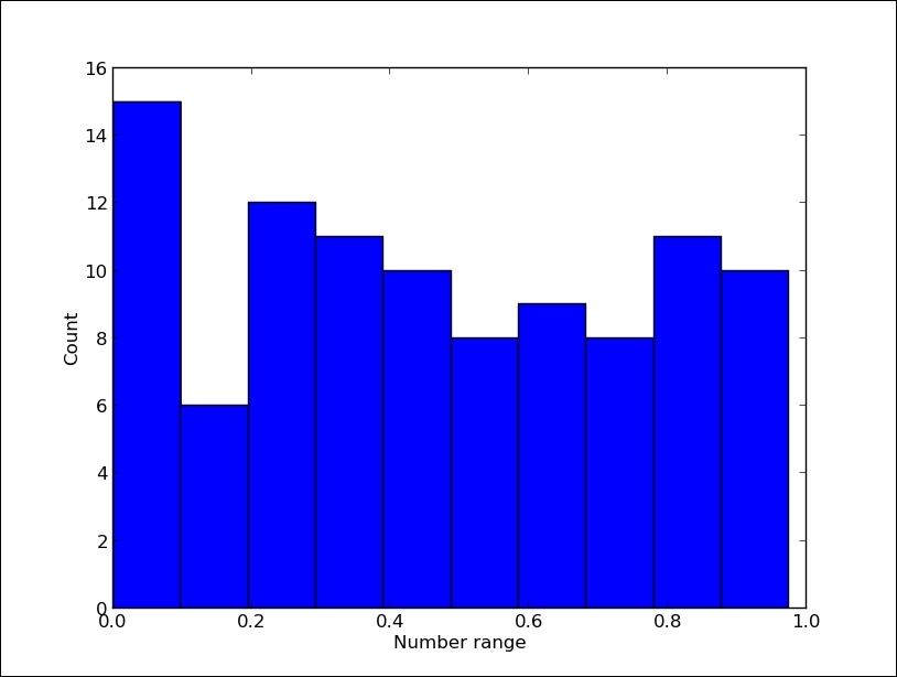
pylab.show()

This is a uniformly distributed sample. When we run this example, we should see something similar to the following plot:

Try setting SAMPLE_SIZE to a big number (say 10000) and see how the histogram behaves.

If we want to have values that range not from 0 to 1, but say from 1 to 6 (by simulating single dice throws), we could use random.randint(min, max); here, min and max are the lower and upper inclusive bounds respectively. If what you want to generate are floats and not integers, there is a random.uniform(min, max) function to provide that.

In a similar fashion and using the same tools, we can generate a time series plot of fictional price growth data with some random noise, as shown here:

import pylab
import random

# days to generate data for
duration = 100
# mean value
mean_inc = 0.2

# standard deviation
std_dev_inc = 1.2

# time series
x = range(duration)
y = []
price_today = 0

for i in x:
    next_delta = random.normalvariate(mean_inc, std_dev_inc)
    price_today += next_delta
    y.append(price_today)

pylab.plot(x,y)
pylab.xlabel("Time")
pylab.xlabel("Time")
pylab.ylabel("Value")
pylab.show()

This code defines a series of 100 data points (fictional days). For every next day, we pick a random value from the normal distribution (random.normalvariate()) ranging from mean_inc to std_dev_inc and add that value to yesterday's price value (price_today).

If we wanted more control, we could use different distributions. The following code illustrates and visualizes different distributions. We will comment separate code sections as we present them. We start by importing required modules and defining a number of histogram buckets. We also create a figure that will hold our histograms as shown in the following lines of code:

# coding: utf-8
import random
import matplotlib
import matplotlib.pyplot as plt

SAMPLE_SIZE = 1000
# histogram buckets
buckets = 100

plt.figure()

# we need to update font size just for this example
matplotlib.rcParams.update({'font.size': 7})

To lay out all the required plots, we define a grid of six by two subplots for all the histograms. The first plot is a uniformly distributed random variable as seen in the following lines of code:

plt.subplot(621)
plt.xlabel("random.random")
# Return the next random floating point number in the range [0.0, 1.0).
res = [random.random() for _ in xrange(1, SAMPLE_SIZE)]
plt.hist(res, buckets)

For the second plot, we plot a uniformly distributed random variable as shown here:

plt.subplot(622)
plt.xlabel("random.uniform")
# Return a random floating point number N such that a <= N <= b for a <= b and b <= N <= a for b < a.
# The end-point value b may or may not be included in the range depending on floating-point rounding in the equation a + (b-a) * random().
a = 1
b = SAMPLE_SIZE
res = [random.uniform(a, b) for _ in xrange(1, SAMPLE_SIZE)]
plt.hist(res, buckets)

Here is the third plot which is a triangular distribution:

plt.subplot(623)
plt.xlabel("random.triangular")

# Return a random floating point number N such that low <= N <= high and with the specified  # mode between those bounds. The low and high bounds default to zero and one. The mode 
# argument defaults to the midpoint between the bounds, giving a symmetric distribution.
low = 1
high = SAMPLE_SIZE
res = [random.triangular(low, high) for _ in xrange(1, SAMPLE_SIZE)]
plt.hist(res, buckets)

The fourth plot is a beta distribution. The condition on the parameters is that alpha and beta should be greater than zero. The returned values range between 0 and 1.

plt.subplot(624)
plt.xlabel("random.betavariate")
alpha = 1
beta = 10
res = [random.betavariate(alpha, beta) for _ in xrange(1, SAMPLE_SIZE)]
plt.hist(res, buckets)

The fifth plot visualizes an exponential distribution. lambd is 1.0 divided by the desired mean. It should be non-zero (the parameter would be called lambda, but that is a reserved word in Python). The returned values range from 0 to positive infinity if lambd is positive, and from negative infinity to 0 if lambd is negative, as shown here:

plt.subplot(625)
plt.xlabel("random.expovariate")
lambd = 1.0 / ((SAMPLE_SIZE + 1) / 2.)
res = [random.expovariate(lambd) for _ in xrange(1, SAMPLE_SIZE)]
plt.hist(res, buckets)

Our next plot is the gamma distribution, where the condition on the parameters is that alpha and beta are greater than 0. The probability distribution function is shown here:

Here's the code for the gamma distribution:

plt.subplot(626)
plt.xlabel("random.gammavariate")


alpha = 1
beta = 10
res = [random.gammavariate(alpha, beta) for _ in xrange(1, SAMPLE_SIZE)]
plt.hist(res, buckets)

Log normal distribution is our next plot. If you take the natural logarithm of this distribution, you'll get a normal distribution with the mean mu and the standard deviation sigma. mu can have any value; moreover, sigma must be greater than zero as shown here:

plt.subplot(627)
plt.xlabel("random.lognormvariate")
mu = 1
sigma = 0.5
res = [random.lognormvariate(mu, sigma) for _ in xrange(1, SAMPLE_SIZE)]
plt.hist(res, buckets)

The next plot is normal distribution, where mu is the mean and sigma is the standard deviation as shown here:

plt.subplot(628)
plt.xlabel("random.normalvariate")
mu = 1
sigma = 0.5
res = [random.normalvariate(mu, sigma) for _ in xrange(1, SAMPLE_SIZE)]
plt.hist(res, buckets)

Here is the last plot which is the Pareto distribution and alpha is the shape parameter:

plt.subplot(629)
plt.xlabel("random.paretovariate")
alpha = 1
res = [random.paretovariate(alpha) for _ in xrange(1, SAMPLE_SIZE)]
plt.hist(res, buckets)

plt.tight_layout()
plt.show()

This was a big code example, but basically we pick 1,000 random numbers according to various distributions. These are common distributions used in different statistical branches (economics, sociology, bio-sciences, and so on).

We should see differences in the histogram based on the distribution algorithm used. Take a moment to understand the following nine plots:

Use seed() to initialize the pseudo-random generator, so random() produces the same expected random values. This is sometimes useful and it is better than pregenerating random data and saving it to a file. The latter technique is not always feasible as it requires saving (possibly huge amounts of) data on a filesystem.

If you want to prevent any repeatability of your randomly generated sequences, we recommend using random.SystemRandom, which uses os.urandom underneath; os.urandom provides access to more entropy sources. If using this random generator interface, seed() and setstate() have no effect; hence these samples are not reproducible.

If we want to have some random words, the easiest way (on Linux) is probably to use /usr/share/dicts/words. We can see how that is done in the following example:

import random

with open('/usr/share/dict/words', 'rt') as f:
    words = f.readlines()
words = [w.rstrip() for w in words]

for w in random.sample(words, 5):
    print w

This solution is for Unix only and will not work on Windows (but, it will work on Mac OS). For Windows, you could use a file constructed from various free sources (Project Gutenberg, Wiktionary, British National Corpus, or http://norvig.com/big.txt by Dr Peter Norvig).