
In Chapter 2, Data Processing Pipeline Using Scala, we discussed different kinds of data types – continuous, discrete, and so on – and a couple of data cleaning methods. Now is the time to see what else we can do for cleaning and extraction of data. Spark provides many approaches for feature extraction and transformation: TF-IDF, Word2Vec, StandardScaler, normalizer, and feature selection.
TF (short for term frequency) and IDF (short for inverted document
frequency). TF-IDF is specifically suited for text documents where we determine the discriminating power of a term in a document using this score. In Spark, TF can be calculated using HashingTF, which is based on a hashing trick and it uses less space when compared with the total possible number of terms present in all documents. On the other hand, IDF is calculated after we have determined TFs for all the documents. So essentially, it captures the essence of word count statistics among all the documents and also preserves the discriminating power of different words across all documents. Mathematically, TF-IDF for a term t, occurring in a document d, can be written as:
Where 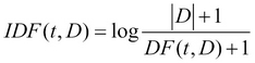 :
:
 is the set of documents
 is the total number of documents
 is the TF
There can be many variations of a TF-IDF formula, however this is the one used in Spark implementation right now.
The following graph depicts the power of TF-IDF, such that we can now use it to distinguish among stop-words, frequent-words, and rare-words:

One of the approaches to turn text data into vector representation is to use Word2Vec, which creates a vector representation of words in a text corpus. In Spark, a skip-gram model is used using the hierarchical softmax method to train these vectors. This vector representation can be used in performing Natural Language Processing (NLP) and for ML algorithms.
Word2Vec basically creates vectors for all words in a text corpus based on the context in which it occurs. Given these vectors you can make queries for a given word, and the Word2Vec model will return words which are synonymous in meaning. This is amazing because the algorithm doesn't really understand any grammar or meanings of words but is still capable of giving pretty sensible results. For example, you can look at an example on Spark documentation here: https://spark.apache.org/docs/1.4.1/mllib-feature-extraction.html#word2vec. When you generate a model for text8 corpus, you can make a query for India and this is what you will get:
scala> val synonyms = sameModel.findSynonyms("india", 5)
synonyms: Array[(String, Double)] = Array((pakistan,1.6807150073221284), (nepal,1.5295662756996018), (tibet,1.5212651063129028), (indonesia,1.5115830206114467), (gujarat,1.4644601715558132))

scala> for((synonym, cosineSimilarity) <- synonyms) {println(s"$synonym $cosineSimilarity")}
pakistan 1.6807150073221284
nepal 1.5295662756996018
tibet 1.5212651063129028
indonesia 1.5115830206114467
gujarat 1.4644601715558132
That is the power of Word2Vec. For more extensive details and use cases of Word2Vec please watch this video: https://www.youtube.com/watch?v=vkfXBGnDplQ.
In Chapter 2, Data Processing Pipeline Using Scala, we discussed what standardization means. Standardizing all the features on a common scale avoids the influence of features with high variance on the rest of the features, thereby also influencing the behavior of the final model. Spark provides StandardScaler and StandardScalerModel classes for performing standardization on the dataset.
We also discussed normalization in Chapter 2, Data Processing Pipeline Using Scala. Normalization is specifically more suited for vector space models, where we are only interested in the angle between two vectors. Spark provides a normalizer class for this task.
As the number of features increases, the requirement for the size of data to backup quality results also increases. This is also called the curse of dimensionality. So by feature selection we choose which of the features we want to select to create a NL model. Feature selection is best done by having some domain knowledge. For example, if you have two features "total price" and "total sales tax," then one of them is redundant because the "percentage sales tax" is always fixed. So we can infer one from the other. Also, we perform correlation analysis on these two features; we will get a high correlation score. Spark provides Chi-squared feature selection to help us with this task. Also, note that as we decrease the number of features via feature selection, we are not degrading the quality of results. We are only selecting the relevant features for the given ML task – in a sense we are reducing the dimensionality of the dataset. Chi-squared is done using ChiSquaredSelector class in Spark. There is another approach called dimensionality reduction that we will see next.
Spark provides us with two ways of performing dimensionality reduction: SVD and PCA. SVD (short for Singular Values Decomposition) is a matrix factorization approach where a given matrix can be decomposed into three matrices that satisfy the following equation:
Where:
- U contains left singular vectors
- V contains right singular vectors
 is a diagonal matrix with singular values on the diagonal
Now, after we perform SVD, and we choose only top k singular values, we can reconstruct the original matrix ![]() .
.
PCA (short for Principal Component Analysis), which is perhaps the most popular form of dimensionality reduction. To appreciate the power of PCA, we must first recall that we should never over-fit our models. The reason is that if we over-fit a model, it will likely produce bad results on an unknown dataset. To overcome this problem, we have to find a training dataset that has most variance, which in turn increases the chances of covering some unknown dataset, however at the same time we want to do that in a reduced dimension. The goal of PCA is to find those projections of the dataset which maximize the variance, and these projections are found in decreasing order of variance. Once we find the projections using PCA, our task is to select the first few projections and use them instead of the original dataset. While PCA is based on statistics, SVD is a numerical method. Although PCA and SVD are excellent tools for dimensionality reduction, one should be careful running them on huge datasets as they are themselves very resource intensive. Therefore, it is best to first apply manual feature selection and then run these algorithms.
Once we have extracted, transformed, and reduced our dataset, it is time to run some ML algorithms on the dataset. In the following sections, we will see the different algorithms provided by Spark.