We now have enough material to enter the heart of the subject. We were able to detect near-duplicate events and group similar articles within a story. In this section, we will be working in real time (on a Spark Streaming context), listening for news articles, grouping them into stories, but also looking at how these stories may change over time. We appreciate that the number of stories is undefined as we do not know in advance what events may arise in the coming days. As optimizing KMeans for each batch interval (15 mn in GDELT) would not be ideal, neither would it be efficient, we decided to take this constraint not as a limiting factor but really as an advantage in the detection of breaking news articles.
If we were to divide the world's news articles into say 10 or 15 clusters, and fix that number to never change over time, then training a KMeans clustering should probably group similar (but not necessarily duplicate) articles into generic stories. For convenience, we give the following definitions:
- An article is the news article covering a particular event at a time T
- A story is a group of similar articles covering an event at a time T
- A topic is a group of similar stories covering different events over a period P
- An epic is a group of similar stories covering the same event over a period P
We assume that after some time without any major news events, any story will be grouped into distinct topics (each covering one or several themes). As an example, any article about politics - regardless the nature of the political event - may be grouped into the politics bucket. This is what we call the Equilibrium state, where the world is equally divided into 15 distinct and clear categories (war, politics, finance, technology, education, and so on).
But what happens if a major event just breaks through? An event may become so important that, over time, (and because of the fixed number of clusters) it could shadow the least important topic and become part of its own topic. Similar to the BBC broadcast that is limited to a 30 mn window, some minor events like the Oyster festival in Whitstable may be skipped in favor of a major international event (to the very dismay of oysters' fans). This topic is not generic anymore but is now associated to a particular event. We called this topic an epic. As an example, the generic topic [terrorism, war, and violence] became an epic [Paris Attacks] in November last year when a major terrorist attack broke through; what was deemed to be a broad discussion about violence and terrorism in general became a branch dedicated to the articles covering the events held in Paris.
Now imagine an epic keeps growing in size; while the first articles about Paris Attacks were covering facts, few hours later, the entire world was paying tribute and condemning terrorism. At the same time, investigations were led by both French and Belgium police to track and dismantle the terrorism network. Both of these stories were massively covered, hence became two different versions of the same epic. This concept of branching is reported in the following Figure 10:

Surely some epics will last longer than others, but when they vanish - if they do - their branches may be recycled to cover new breaking articles (remember the fixed number of clusters) or be re-used to group generic stories back to their generic topics. At some point in time, we eventually reach a new Equilibrium state where the world nicely fits again within 15 different topics. We assume, though, that a new Equilibrium may not be a perfect clone of the previous one as this disturbance may have carved and re-shaped the world somehow. As a concrete example, we still mention 9/11-related articles nowadays; world trade center attacks that happened in NYC in 2001 are still contributing to the definition of [violence, war, and terrorism] topic.
Although the preceding description is more conceptual than anything, and would probably deserve a subject for a PhD in data science applied to geo-politics, we would like to dig that idea further and see how Streaming KMeans could be a fantastic tool for that use case.
The first thing is to acquire our data in real time, hence modifying our existing NiFi flow to fork our downloaded archive to a Spark Streaming context. One could simply netcat the content of a file to an open socket, but we want this process to be resilient and fault tolerant. NiFi comes, by default, with the concept of output ports that provide a mechanism to transfer data to remote instances using Site-To-Site. In that case, the port works like a queue, and no data should be lost in transit, hopefully. We enable this functionality in the nifi.properties file by allocating a port number.
nifi.remote.input.socket.port=8055
We create a port called [Send_To_Spark] on our canvas, and every record (hence the SplitText processor) will be sent to it just like we would be doing on a Kafka topic.

Tip
Although we are designing a streaming application, it is recommended to always keep an immutable copy of your data in a resilient data store (HDFS here). In our NiFi flow earlier, we did not modify our existing process, but forked it to also send records to our Spark Streaming. This will be particularly useful when/if we need to replay part of our dataset.
On the Spark side, we need to build a Nifi receiver. This can be achieved using the following maven dependency:
<dependency>
  <groupId>org.apache.nifi</groupId>
  <artifactId>nifi-spark-receiver</artifactId>
  <version>0.6.1</version>
</dependency>
We define the NiFi endpoint together with the port name [Send_To_Spark] we assigned earlier. Our stream of data will be received as packet stream that can easily be converted into a String using the getContent method.
def readFromNifi(ssc: StreamingContext): DStream[String] = {

  val nifiConf = new SiteToSiteClient.Builder()
    .url("http://localhost:8090/nifi")
    .portName("Send_To_Spark")
    .buildConfig()

  val receiver = new NiFiReceiver(nifiConf, StorageLevel.MEMORY_ONLY)
  ssc.receiverStream(receiver) map {packet =>
    new String(packet.getContent, StandardCharsets.UTF_8)
  }
}
We start our streaming context and listen to new GDELT data coming every 15 mn.
val ssc = new StreamingContext(sc, Minutes(15))
val gdeltStream: DStream[String] = readFromNifi(ssc)
val gkgStream = parseGkg(gdeltStream)
The next step is to download the HTML content for each article. The tricky part here is to download articles for distinct URLs only. As there is no built-in distinct operation on DStream, we need to access the underlying RDDs using a transform operation on top of which we pass an extractUrlsFromRDD function:
val extractUrlsFromRDD = (rdd: RDD[GkgEntity2]) => {
  rdd.map { gdelt =>
    gdelt.documentId.getOrElse("NA")
  }
  .distinct()
}
val urlStream = gkgStream.transform(extractUrlsFromRDD)
val contentStream = fetchHtml(urlStream)
Similarly, building vectors requires access to the underlying RDDs as we need to count the document frequency (used for TF-IDF) across the entire batch. This is also done within the transform function.
val buildVectors = (rdd: RDD[Content]) => {

  val corpusRDD = rdd.map(c => (c, Tokenizer.stem(c.body)))

  val tfModel = new HashingTF(1 << 20)
  val tfRDD = corpusRDD mapValues tfModel.transform

  val idfModel = new IDF() fit tfRDD.values
  val idfRDD = tfRDD mapValues idfModel.transform

  val normalizer = new Normalizer()
  val sparseRDD = idfRDD mapValues normalizer.transform

  val embedding = Embedding(Embedding.MEDIUM_DIMENSIONAL_RI)
  val denseRDD = sparseRDD mapValues embedding.embed

  denseRDD
}

val vectorStream = contentStream transform buildVectorsOur use case perfectly fits in a Streaming KMeans algorithm. The concept of Streaming KMeans does not differ from the classic KMeans except that it applies on dynamic data and therefore needs to be constantly re-trained and updated.
At each batch, we find the closest center for each new data point, average the new cluster centers and update our model. As we track the true clusters and adapt to the changes in pseudo real-time, it will be particularly easy to track the same topics across different batches.
The second important feature of a Streaming KMeans is the forgetfulness. This ensures new data points received at time t will be contributing more to the definition of our clusters than any other point in the past history, hence allowing our cluster centers to smoothly drift over time (stories will mutate). This is controlled by the decay factor and its half-life parameter (expressed in the number of batches or number of points) that specifies the time after which a given point will only contribute half of its original weight.
- With an infinite decay factor, all the history will be taken into account, our cluster centers will be drifting slowly and will not be reactive if a major news event just breaks through
- With a small decay factor, our clusters will be too reactive towards any point and may drastically change any time a new event is observed
The third and most important feature of a Streaming KMeans is the ability to detect and recycle dying clusters. When we observe a drastic change in our input data, one cluster may become far from any known data point. Streaming KMeans will eliminate this dying cluster and split the largest one in two. This is totally in-line with our concept of story branching, where multiple stories may share a common ancestor.
We use a half-life parameter of two batches here. As we get new data every 15 mn, any new data point will stay active for 1 hour only. The process for training Streaming KMeans is reported in Figure 12:

We create a new Streaming KMeans as follows. Because we did not observe any data point yet, we initialize it with 15 random centers of 256 large vectors (size of our TF-IDF vectors) and train it in real time using the trainOn method:
val model = new StreamingKMeans()
  .setK(15)
  .setRandomCenters(256, 0.0)
  .setHalfLife(2, "batches")

model.trainOn(vectorStream.map(_._2))
Finally, we predict our clusters for any new data point:
val storyStream = model predictOnValues vectorStream
We then save our results to our Elasticsearch cluster using the following attributes (accessed through a series of join operations). We do not report here how to persist RDD to Elasticsearch as we believe this has been covered in depth in the previous chapters already. Note that we also save the vector itself as we may re-use it later in the process.
Map(
  "uuid" -> gkg.gkgId,
  "topic" -> clusterId,
  "batch" -> batchId,
  "simhash" -> content.body.simhash,
  "date" -> gkg.date,
  "url" -> content.url,
  "title" -> content.title,
  "body" -> content.body,
  "tone" -> gkg.tones.get.averageTone,
  "country" -> gkg.v2Locations,
  "theme" -> gkg.v2Themes,
  "person" -> gkg.v2Persons,
  "organization" -> gkg.v2Organizations,
  "vector" -> v.toArray.mkString(",")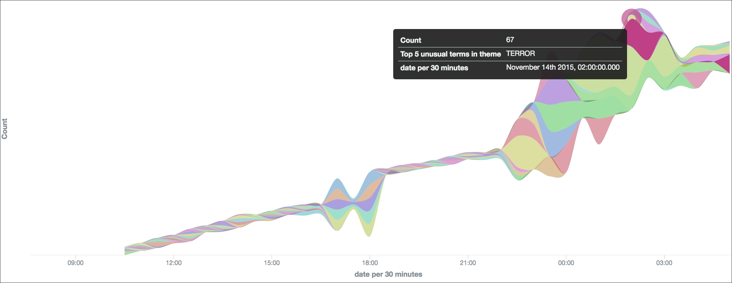
)As we stored our articles with their respective stories and topics on Elasticsearch, we can browse any events using a keyword search (as the articles are fully analyzed and indexed) or for a particular person, theme, organization, and so on. We build visualizations on top of our stories and try to detect their potential drifts on a Kibana dashboard. The different cluster IDs (our different topics) over time are reported in the following Figure 13 for the 13th of November (35,000 articles indexed):

The results are quite promising. We were able to detect the Paris Attacks at around 9:30 p.m. on November 13th, only a few minutes after the first attacks started. We also confirm a relative good consistency of our clustering algorithm as a particular cluster was made of events related to the Paris Attacks only (5,000 articles) from 9:30 p.m. to 3:00 a.m.
But we may wonder what this particular cluster was about before the first attack took place. Since we indexed all the articles together with their cluster ID and their GKG attributes, we can easily track a story backwards in time and detect its mutation. It turns out this particular topic was mainly covering events related to [MAN_MADE_DISASTER] theme (among others) until 9 p.m. to 10 p.m. when it turned into the Paris Attacks epic with themes around [TERROR], [STATE_OF_EMERGENCY], [TAX_ETHNICITY_FRENCH], [KILL], and [EVACUATION].
Needless to say the 15 mn average tone we get from GDELT dropped drastically after 9 p.m. for that particular topic:

Using these three simple visualizations, we prove that we can track a story over time and study its potential mutation in genre, keywords, persons, or organizations (basically any entity we can extract from GDELT). But we could also look at the geolocation from the GKG records; with enough articles, we could possibly track the terrorist hunt held between Paris and Brussels on a map, in pseudo real time!
Although we found one main cluster that was specific to the Paris Attacks, and that this particular cluster was the first one to cover this series of events, this may not be the only one. According to the Streaming KMeans definition earlier, this topic became so big that it surely had triggered one or several subsequent epics. We report in the following Figure 16 the same results as per Figure 13, but this time filtered out for any article matching the keyword Paris:

It seems that around midnight, this epic gave rise to multiple versions of the same event (at least three major ones). After an hour following the attacks (1 hour is our decay factor), Streaming KMeans started to recycle dying clusters, hence creating new branches out of the most important event (our Paris attack cluster).
While the main epic was still covering the event itself (the facts), the second most important one was more about social network related articles. A simple word frequency analysis tells us this epic was about the #portesOuvertes (open doors) and #prayForParis hashtags where Parisians responded to terror with solidarity. We also detected another cluster focusing more on all the politicians paying tributes to France and condemning terrorism. All these new stories share the Paris attack epic as a common ancestor, but cover a different flavor of it.
How can we link these branches together? How can we track an epic over time and see when, if, how, or why it may split? Surely visualization helps, but we are looking at a graph problem to solve here.
Because our KMeans model keeps getting updated at each batch, our approach is to retrieve the articles that we predicted using an outdated version of our model, pull them from Elasticsearch, and predict them against our updated KMeans. Our assumption is as follows:
If we observe many articles at a time t that belonged to a story s, and now belong to a story s' at a time ![]() , then s
most likely migrated to s' in
, then s
most likely migrated to s' in ![]() time.
time.
As a concrete example, the first #prayForParis article was surely belonging to the Paris Attacks epic. Few batches later, that same article belonged to the Paris Attacks/Social Network cluster. Therefore, the Paris Attack epic may have spawn the Paris Attacks/Social Network epic. This process is reported in the following Figure 17:

We read a JSON RDD from Elasticsearch and applied a range query using the batch ID. In the following example, we want to access all the vectors built over the past hour (four last batches) together with their original cluster ID and re-predict them against our updated model (accessed through the latestModel function):
import org.json4s.DefaultFormats
import org.json4s.native.JsonMethods._

val defaultVector = Array.fill[Double](256)(0.0d).mkString(",")
val minBatchQuery = batchId - 4
val query = "{"query":{"range":{"batch":{"gte": " + minBatchQuery + ","lte": " + batchId + "}}}}"
val nodesDrift = sc.esJsonRDD(esArticles, query)
  .values
  .map { strJson =>
    implicit val format = DefaultFormats
    val json = parse(strJson)
    val vectorStr = (json  "vector").extractOrElse[String](defaultVector)
    val vector = Vectors.dense(vectorStr.split(",").map(_.toDouble))
    val previousCluster = (json  "topic").extractOrElse[Int](-1)
    val newCluster = model.latestModel().predict(vector)
    ((previousCluster, newCluster), 1)
  }
  .reduceByKey(_ + _)
Finally, a simple reduceByKey function will count the number of different edges over the past hour. In most of the cases, articles in story s will stay in story s, but in case of the Paris attacks, we may observe some stories to drift over time towards different epics. Most importantly, the more connections two branches have in common, the more similar they are (as many of their articles are interconnected) and therefore the closest they seem to be in a force directed layout. Similarly, branches that are not sharing many connections will seem to be far from another in the same graph visualization. A force atlas representation of our story connections is done using Gephi software and reported in the following Figure 18. Each node is a story at a batch b, and each edge is the number of connections we found between two stories. The 15 lines are our 15 topics that all share a common ancestor (the initial cluster spawn when first starting the streaming context).

The first observation we can make is this line shape. This observation surprisingly confirms our theory of an Equilibrium state where the world nicely fitted in 15 distinct topics until the Paris attacks happened. Before the event, most of the topics were isolated and intraconnected (hence this line shape). After the event, we see our main Paris Attack epic to be dense, interconnected, and drifting over time. It also seems to drag few branches down with it due to the growing number on interconnections. These two similar branches are the two other clusters mentioned earlier (social network and tributes). This epic is being more and more specific over time, it naturally becomes more different from others, hence pushing all these different stories upwards and resulting in this scatter shape.
We also want to know what these different branches were about, and whether or not we could explain why a story may have split into two. For that purpose, we find the main article of each story as being the closest point to its centroid.
val latest = model.latestModel()
val topTitles = rdd.values
  .map { case ((content, v, cId), gkg) =>
    val dist = euclidean(
                  latest.clusterCenters(cId).toArray,
                  v.toArray
                  )
    (cId, (content.title, dist))
  }
  .groupByKey()
  .mapValues { it =>
    Try(it.toList.sortBy(_._2).map(_._1).head).toOption
  }
  .collectAsMap()
In Figure 19, we report the same graph enriched with the story titles. Although it is difficult to find a clear pattern, we found an interesting case. A topic was covering (among others) an event related to Prince Harry joking around about his hair style, that slightly migrated to Obama offering a statement on the attack in Paris, and finally turned into the Paris attack and the tributes paid by politicians. This branch did not come out of nowhere but seemed to follow a logical flow:
- [ROYAL, PRINCE HARRY, JOKES]
- [ROYAL, PRINCE HARRY]
- [PRINCE HARRY, OBAMA]
- [PRINCE HARRY, OBAMA, POLITICS]
- [OBAMA, POLITICS]
- [OBAMA, POLITICS, PARIS]
- [POLITICS, PARIS]

To summarize, it seems that a breaking news event acts as a sudden perturbation of an Equilibrium state. Now we may wonder how long would that disturbance last, whether or not a new Equilibrium will be reached in the future and what would be the shape of the world resulting from that wound. Most importantly, what effect a different decay factor would have on that world shape.
With enough time and motivation, we would potentially be interested in applying some concepts of physics around perturbation theory (http://www.tcm.phy.cam.ac.uk/~bds10/aqp/handout_dep.pdf). I personally would be interested in finding harmonics around this Equilibrium. The reason of the Paris attacks events being so memorable is because of its violent nature for sure, but also because it happened only a few months after the Charlie Hebdo attacks in Paris.