
Most of the data comes in a very unpractical form for applying machine-learning algorithms. As we have seen in the example (in the preceding paragraph), the data can have missing values or non-numeric columns, which are not ready to be fed into any machine-learning technique. Therefore, a machine-learning professional usually spends a large amount of time cleaning and preparing the data to transform it into a form suitable for further analysis or visualization. This section will teach how to use numpy and pandas to create, prepare, and manipulate data in Python while the matplotlib paragraph will provide the basis of plotting a graph in Python. The Python shell has been used to discuss the NumPy tutorial, although all versions of the code in the IPython notebook, and plain Python script, are available in the chapter_1 folder of the author's GitHub. pandas and matplotlib are discussed using the IPython notebook.
Numerical Python or NumPy, is an open source extension library for Python, and is a fundamental module required for data analysis and high performance scientific computing. The library features support Python for large, multi-dimensional arrays and matrices, and it provides precompiled functions for numerical routines. Furthermore, it provides a large library of mathematical functions to manipulate these arrays.
The library provides the following functionalities:
- Fast multi-dimensional array for vector arithmetic operations
- Standard mathematical functions for fast operations on entire arrays of data
- Linear algebra
- Sorting, unique, and set operations
- Statistics and aggregating data
The main advantage of NumPy is the speed of the usual array operations compared to standard Python operations. For instance, a traditional summation of 10000000 elements:
>>> def sum_trad():
>>>   start = time.time()
>>>   X = range(10000000)
>>>   Y = range(10000000)
>>>   Z = []
>>>   for i in range(len(X)):
>>>       Z.append(X[i] + Y[i])
>>>   return time.time() - start
Compare this to the Numpy function:
>>> def sum_numpy():
>>>
start = time.time()
>>>   X = np.arange(10000000)
>>>   Y = np.arange(10000000)
>>>   Z=X+Y
>>>   return time.time() - start
>>> print 'time sum:',sum_trad(),'  time sum numpy:',sum_numpy()
time sum: 2.1142539978   time sum numpy: 0.0807049274445
The time used is 2.1142539978 and 0.0807049274445 respectively.
The array object is the main feature provided by the NumPy library. Arrays are the equivalent of Python lists, but each element of an array has the same numerical type (typically float or int). It is possible to define an array casting from a list using the function array by using the following code. Two arguments are passed to it: the list to be converted and the type of the new generated array:
>>> arr = np.array([2, 6, 5, 9], float)
>>> arr
array([ 2., 6., 5., 9.])
>>> type(arr)
<type 'numpy.ndarray'>
And vice versa, an array can be transformed into a list by the following code:
>>> arr = np.array([1, 2, 3], float)
>>> arr.tolist()
[1.0, 2.0, 3.0]
>>> list(arr)
[1.0, 2.0, 3.0]
To create a new object from an existing one, the copy function needs to be used:
>>> arr = np.array([1, 2, 3], float)
>>> arr1 = arr
>>> arr2 = arr.copy()
>>> arr[0] = 0
>>> arr
array([0., 2., 3.])
>>> arr1
array([0., 2., 3.])
>>> arr2
array([1., 2., 3.])
Alternatively an array can be filled with a single value in the following way:
>>> arr = np.array([10, 20, 33], float)
>>> arr
array([ 10., 20., 33.])
>>> arr.fill(1)
>>> arr
array([ 1., 1., 1.])
Arrays can also be created randomly using the random submodule. For example, giving the length of an array as an input of the function, permutation will find a random sequence of integers:
>>> np.random.permutation(3)
array([0, 1, 2])
Another method, normal, will draw a sequence of numbers from a normal distribution:
>>> np.random.normal(0,1,5)
array([-0.66494912,  0.7198794 , -0.29025382,  0.24577752,  0.23736908])
0 is the mean of the distribution while 1 is the standard deviation and 5 is the number of array's elements to draw. To use a uniform distribution, the random function will return numbers between 0 and 1 (not included):
>>> np.random.random(5)
array([ 0.48241564,  0.24382627,  0.25457204,  0.9775729 ,  0.61793725])
NumPy also provides a number of functions for creating two-dimensional arrays (matrices). For instance, to create an identity matrix of a given dimension, the following code can be used:
>>> np.identity(5, dtype=float)
array([[ 1.,  0.,  0.,  0.,  0.],
       [ 0.,  1.,  0.,  0.,  0.],
       [ 0.,  0.,  1.,  0.,  0.],
       [ 0.,  0.,  0.,  1.,  0.],
       [ 0.,  0.,  0.,  0.,  1.]])
The eye function returns matrices with ones along the kth diagonal:
>>> np.eye(3, k=1, dtype=float)
array([[ 0.,  1.,  0.],
       [ 0.,  0.,  1.],
       [ 0.,  0.,  0.]])
The most commonly used functions to create new arrays (1 or 2 dimensional) are zeros and ones which create new arrays of specified dimensions filled with these values. These are:
>>> np.ones((2,3), dtype=float)
array([[ 1., 1., 1.],
       [ 1., 1., 1.]])
>>> np.zeros(6, dtype=int)
array([0, 0, 0, 0, 0, 0])
The zeros_like and ones_like functions instead create a new array with the same type as an existing one, with the same dimensions:
>>> arr = np.array([[13, 32, 31], [64, 25, 76]], float)
>>> np.zeros_like(arr)
array([[ 0.,  0.,  0.],
       [ 0.,  0.,  0.]])
>>> np.ones_like(arr)
array([[ 1.,  1.,  1.],
       [ 1.,  1.,  1.]])
Another way to create two-dimensional arrays is to merge one-dimensional arrays using vstack (vertical merge):
>>> arr1 = np.array([1,3,2])
>>> arr2 = np.array([3,4,6])
>>> np.vstack([arr1,arr2])
array([[1, 3, 2],
       [3, 4, 6]])
The creation using distributions are also possible for two-dimensional arrays, using the random submodule. For example, a random matrix 2x3 from a uniform distribution between 0 and 1 is created by the following command:
>>> np.random.rand(2,3)
array([[ 0.36152029,  0.10663414,  0.64622729],
    [ 0.49498724,  0.59443518,  0.31257493]])
Another often used distribution is the multivariate normal distribution:
>>> np.random.multivariate_normal([10, 0], [[3, 1], [1, 4]], size=[5,])
array([[ 11.8696466 ,  -0.99505689],
       [ 10.50905208,   1.47187705],
       [  9.55350138,   0.48654548],
       [ 10.35759256,  -3.72591054],
       [ 11.31376171,   2.15576512]])
The list [10,0] is the mean vector, [[3, 1], [1, 4]] is the covariance matrix and 5 is the number of samples to draw.
All the usual operations to access, slice, and manipulate a Python list can be applied in the same way, or in a similar way to an array:
>>> arr = np.array([2., 6., 5., 5.])
>>> arr[:3]
array([ 2., 6., 5.])
>>> arr[3]
5.0
>>> arr[0] = 5.
>>> arr
array([ 5., 6., 5., 5.])
The unique value can be also selected using unique:
>>> np.unique(arr)
array([ 5., 6., 5.])
The values of the array can also be sorted using sort and its indices with argsort:
>>> np.sort(arr)
array([ 2.,  5.,  5.,  6.])
>>> np.argsort(arr)
array([0, 2, 3, 1])
It is also possible to randomly rearrange the order of the array's elements using the shuffle function:
>>> np.random.shuffle(arr)
>>> arr
array([ 2.,  5.,  6.,  5.])
NumPy also has a built-in function to compare arrays array_equal:
>>> np.array_equal(arr,np.array([1,3,2]))
False
Multi-dimensional arrays, however, differ from the list. In fact, a list of dimensions is specified using the comma (instead of a bracket for list). For example, the elements of a two-dimensional array (that is a matrix) are accessed in the following way:
>>> matrix = np.array([[ 4., 5., 6.], [2, 3, 6]], float)
>>> matrix
array([[ 4., 5., 6.],
       [ 2., 3., 6.]])
>>> matrix[0,0]
4.0
>>> matrix[0,2]
6.0
Slicing is applied on each dimension using the colon : symbol between the initial value and the end value of the slice:
>>> arr = np.array([[ 4., 5., 6.], [ 2., 3., 6.]], float)
>>> arr[1:2,2:3]
array([[ 6.]])
While a single : means all the elements along that axis are considered:
>>> arr[1,:]
array([2, 3, 6])
>>> arr[:,2]
array([ 6., 6.])
>>> arr[-1:,-2:]
array([[ 3., 6.]])
One-dimensional arrays can be obtained from multi-dimensional arrays using the flatten function:
>>> arr = np.array([[10, 29, 23], [24, 25, 46]], float)
>>> arr
array([[ 10.,  29.,  23.],
       [ 24.,  25.,  46.]])
>>> arr.flatten()
array([ 10.,  29.,  23.,  24.,  25.,  46.])
It is also possible to inspect an array object to obtain information about its content. The size of an array is found using the attribute shape:
>>> arr.shape
(2, 3)
In this case, arr is a matrix of two rows and three columns. The dtype property returns the type of values are stored within the array:
>>> arr.dtype
dtype('float64')
float64 is a numeric type to store double-precision (8-byte) real numbers (similar to float type in regular Python). There are also other data types such as int64, int32, string, and an array can be converted from one type to another. For example:
>>>int_arr = matrix.astype(np.int32)
>>>int_arr.dtype
dtype('int32')
The len function returns the length of the first dimension when used on an array:
>>>arr = np.array([[ 4., 5., 6.], [ 2., 3., 6.]], float)
>>> len(arr)
2
Like in Python for loop, the in word can be used to check if a value is contained in an array:
>>> arr = np.array([[ 4., 5., 6.], [ 2., 3., 6.]], float)
>>> 2 in arr
True
>>> 0 in arr
False
An array can be manipulated in such a way that its elements are rearranged in different dimensions using the function reshape. For example, a matrix with eight rows and one column can be reshaped to a matrix with four rows and two columns:
>>> arr = np.array(range(8), float)
>>> arr
array([ 0., 1., 2., 3., 4., 5., 6., 7.])
>>> arr = arr.reshape((4,2))
>>> arr
array([[ 0.,  1.],
       [ 2.,  3.],

[ 4.,  5.],
       [ 6.,  7.]])
>>> arr.shape
(4, 2)
In addition, transposed matrices can be created; that is to say, a new array with the final two dimensions switched can be obtained using the transpose function:
>>> arr = np.array(range(6), float).reshape((2, 3))
>>> arr
array([[ 0., 1., 2.],
      [ 3., 4., 5.]])
>>> arr.transpose()
array([[ 0., 3.],
       [ 1., 4.],
       [ 2., 5.]])
Arrays can also be transposed using the T attribute:
>>> matrix = np.arange(15).reshape((3, 5))
>>> matrix
array([[ 0, 1, 2, 3, 4],
       [ 5, 6, 7, 8, 9],
       [10, 11, 12, 13, 14]])
>>>matrix .T
array([[ 0, 5, 10],
       [ 1, 6, 11],
       [ 2, 6, 12],

[ 3, 8, 13],
       [ 4, 9, 14]])
Another way to reshuffle the elements of an array is to use the newaxis function to increase the dimensionality:
>>> arr = np.array([14, 32, 13], float)
>>> arr
array([ 14.,  32.,  13.])
>> arr[:,np.newaxis]
array([[ 14.],
       [ 32.],
       [ 13.]])
>>> arr[:,np.newaxis].shape
(3,1)
>>> arr[np.newaxis,:]
array([[ 14.,  32.,  13.]])
>>> arr[np.newaxis,:].shape
(1,3)
In this example, in each case the new array has two dimensions, the one generated by newaxis has a length of one.
Joining arrays is an operation performed by the concatenate function in NumPy, and the syntax depends on the dimensionality of the array. Multiple one-dimensional arrays can be chained, specifying the arrays to be joined as a tuple:
>>> arr1 = np.array([10,22], float)
>>> arr2 = np.array([31,43,54,61], float)
>>> arr3 = np.array([71,82,29], float)
>>> np.concatenate((arr1, arr2, arr3))
array([ 10.,  22.,  31.,  43.,  54.,  61.,  71.,  82.,  29.])
Using a multi-dimensional array, the axis along which multiple arrays are concatenated needs to be specified. Otherwise, NumPy concatenates along the first dimension by default:
>>> arr1 = np.array([[11, 12], [32, 42]], float)
>>> arr2 = np.array([[54, 26], [27,28]], float)
>>> np.concatenate((arr1,arr2))
array([[ 11.,  12.],
       [ 32.,  42.],
       [ 54.,  26.],
       [ 27.,  28.]])
>>> np.concatenate((arr1,arr2), axis=0)
array([[ 11.,  12.],
       [ 32.,  42.],
       [ 54.,  26.],
       [ 27.,  28.]])
>>> np.concatenate((arr1,arr2), axis=1)
array([[ 11.,  12.,  54.,  26.],
       [ 32.,  42.,  27.,  28.]])
It is common to save a large amount of data as a binary file instead of using the direct format. NumPy provides a function, tostring, to convert an array to a binary string. Of course there's also the inverse operation, where a conversion of a binary string to an array is supported using the fromstring routine. For example:
>>> arr = np.array([10, 20, 30], float)
>>> str = arr.tostring()
>>> str
'x00x00x00x00x00x00$@x00x00x00x00x00x004@x00x00x00x00x00x00>@'
>>> np.fromstring(str)
array([ 10., 20., 30.])
Common mathematical operations are obviously supported in NumPy. For example:
>>> arr1 = np.array([1,2,3], float)
>>> arr2 = np.array([1,2,3], float)
>>> arr1 + arr2
array([2.,4., 6.])
>>> arr1–arr2
array([0., 0., 0.])
>>> arr1 * arr2
array([51, 4., 9.])
>>> arr2 / arr1
array([1., 1., 1.])
>>> arr1 % arr2
array([0., 0., 0.])
>>> arr2**arr1
array([1., 4., 9.])
Since any operation is applied element wise, the arrays are required to have the same size. If this condition is not satisfied, an error is returned:
>>> arr1 = np.array([1,2,3], float)
>>> arr2 = np.array([1,2], float)
>>> arr1 + arr2
Traceback (most recent call last):
File "<stdin>", line 1, in <module>
ValueError: shape mismatch: objects cannot be broadcast to a single shape
The error states that the objects cannot be broadcasted because the only way to perform an operation with arrays of different size is called broadcasting. This means the arrays have a different number of dimensions, and the array with less dimensions will be repeated until it matches the dimensions of the other array. Consider the following:
>>> arr1 = np.array([[1, 2], [3, 4], [5, 6]], float)
>>> arr2 = np.array([1, 2], float)
>>> arr1
array([[ 1., 2.],
       [ 3., 4.],
       [ 5., 6.]])
>>> arr2
array([1., 1.])
>>> arr1 + arr2
array([[ 2., 4.],
       [ 4., 6.],
       [ 6., 8.]])
The array arr2 was broadcasted to a two-dimensional array that matched the size of arr1. Therefore, arr2 was repeated for each dimension of arr1, equivalent to the array:
array([[1., 2.],[1., 2.],[1., 2.]])
If we want to make the way an array is broadcasted explicit, the newaxis constant allows us to specify how we want to broadcast:
>>> arr1 = np.zeros((2,2), float)
>>> arr2 = np.array([1., 2.], float)
>>> arr1
array([[ 0., 0.],[ 0., 0.]])
>>> arr2
array([1., 2.])
>>> arr1 + arr2
array([[-1., 3.],[-1., 3.]])
>>> arr1 + arr2[np.newaxis,:]
array([[1., 2.],[1., 2.]])
>>> arr1 + arr2[:,np.newaxis]
array([[1.,1.],[ 2., 2.]])
Unlike Python lists, arrays can be queried using conditions. A typical example is to use Boolean arrays to filter the elements:
>>> arr = np.array([[1, 2], [5, 9]], float)
>>> arr >= 7
array([[ False, False],
[False, True]], dtype=bool)
>>> arr[arr >= 7]
array([ 9.])
Multiple Boolean expressions can be used to subset the array:
>>> arr[np.logical_and(arr > 5, arr < 11)]
>>> arr
array([ 9.])
Arrays of integers can be used to specify the indices to select the elements of another array. For example:
>>> arr1 = np.array([1, 4, 5, 9], float)
>>> arr2 = np.array([0, 1, 1, 3, 1, 1, 1], int)
>>> arr1[arr2]
array([ 1., 4., 4., 9., 4., 4., 4.])
The arr2 represents the ordered indices to select elements from array arr1: the zeroth, first, first, third, first, first, and first elements of arr1, in that order have been selected. Also lists can be used for the same purpose:
>>> arr = np.array([1, 4, 5, 9], float)
>>> arr[[0, 1, 1, 3, 1]]
array([ 1., 4., 4., 9., 4.])
In order to replicate the same operation with multi-dimensional arrays, multiple one-dimensional integer arrays have to be put into the selection bracket, one for each dimension.
The first selection array represents the values of the first index in the matrix entries, while the values on the second selection array represent the column index of the matrix entries. The following example illustrates the idea:
>>> arr1 = np.array([[1, 2], [5, 13]], float)
>>> arr2 = np.array([1, 0, 0, 1], int)
>>> arr3 = np.array([1, 1, 0, 1], int)
>>> arr1[arr2,arr3]
array([ 13.,   2.,   1.,  13.])
The values on arr2 are the first index (row) on arr1 entries while arr3 are the second index (column) values, so the first chosen entry on arr1 corresponds to row 1 column 1 which is 13.
The function take can be used to apply your selection with integer arrays, and it works in the same way as bracket selection:
>>> arr1 = np.array([7, 6, 6, 9], float)
>>> arr2 = np.array([1, 0, 1, 3, 3, 1], int)
>>> arr1.take(arr2)
array([ 6.,  7.,  6.,  9.,  9.,  6.])
Subsets of a multi-dimensional array can be selected along a given dimension specifying the axis argument on the take function:
>>> arr1 = np.array([[10, 21], [62, 33]], float)
>>> arr2 = np.array([0, 0, 1], int)
>>> arr1.take(arr2, axis=0)
array([[ 10.,  21.],
       [ 10.,  21.],
       [ 62.,  33.]])
>>> arr1.take(arr2, axis=1)
array([[ 10.,  10.,  21.],
       [ 62.,  62.,  33.]])
The put function is the opposite of the take function, and it takes values from an array and puts them at specified indices in the array that calls the put method:
>>> arr1 = np.array([2, 1, 6, 2, 1, 9], float)
>>> arr2 = np.array([3, 10, 2], float)
>>> arr1.put([1, 4], arr2)
>>> arr1
array([ 2.,  3.,  6.,  2.,  10.,  9.])
We finish this section with the note that multiplication also remains element-wise for two-dimensional arrays (and does not correspond to matrix multiplication):
>>> arr1 = np.array([[11,22], [23,14]], float)
>>> arr2 = np.array([[25,30], [13,33]], float)
>>> arr1 * arr2
array([[ 275.,  660.],
       [ 299.,  462.]])
The most common operations between matrices is the inner product of a matrix with its transpose, XT X, using np.dot:
>>> X = np.arange(15).reshape((3, 5))
>>> X
array([[ 0, 1, 2, 3, 4],
       [ 5, 6, 7, 8, 9],
       [10, 11, 12, 13, 14]])
>>> X.T
array([[ 0, 5, 10],
       [ 1, 6, 11],
       [ 2, 6, 12],
       [ 3, 8, 13],
       [ 4, 9, 14]])
>>>np.dot(X .T, X)#X^T X
array([[ 2.584 , 1.8753, 0.8888],
       [ 1.8753, 6.6636, 0.3884],
       [ 0.8888, 0.3884, 3.9781]])
There are functions to directly calculate the different types of product (inner, outer, and cross) on arrays (that is matrices or vectors).
For one-dimensional arrays (vectors) the inner product corresponds to the dot product:
>>> arr1 = np.array([12, 43, 10], float)
>>> arr2 = np.array([21, 42, 14], float)
>>> np.outer(arr1, arr2)
array([[  252.,   504.,   168.],
       [  903.,  1806.,   602.],
       [  210.,   420.,   140.]])
>>> np.inner(arr1, arr2)
2198.0
>>> np.cross(arr1, arr2)
array([ 182.,   42., -399.])
NumPy also contains a sub-module, linalg that has a series of functions to perform linear algebra calculations over matrices. The determinant of a matrix can be computed as:
>>> matrix = np.array([[74, 22, 10], [92, 31, 17], [21, 22, 12]], float)
>>> matrix
array([[ 74.,  22.,  10.],
       [ 92.,  31.,  17.],
       [ 21.,  22.,  12.]])
>>> np.linalg.det(matrix)
-2852.0000000000032
Also the inverse of a matrix can be generated using the function inv:
>>> inv_matrix = np.linalg.inv(matrix)
>>> inv_matrix
array([[ 0.00070126,  0.01542777, -0.02244039],
       [ 0.26192146, -0.23772791,  0.11851332],
       [-0.48141655,  0.4088359 , -0.09467041]])
>>> np.dot(inv_matrix,matrix)
array([[  1.00000000e+00,   2.22044605e-16,   4.77048956e-17],
       [ -2.22044605e-15,   1.00000000e+00,   0.00000000e+00],
       [ -3.33066907e-15,  -4.44089210e-16,   1.00000000e+00]])
It is straightforward to calculate the eigenvalues and eigenvectors of a matrix:
>>> vals, vecs = np.linalg.eig(matrix)
>>> vals
array([ 107.99587441,   11.33411853,   -2.32999294])
>>> vecs
array([[-0.57891525, -0.21517959,  0.06319955],
       [-0.75804695,  0.17632618, -0.58635713],
       [-0.30036971,  0.96052424,  0.80758352]])
NumPy provides a set of functions to compute statistics of the data contained in the arrays. Operations of the aggregation type, such as sum, mean, median, and standard deviation are available as an attribute of an array. For example, creating a random array (from a normal distribution), it is possible to calculate the mean in two ways:
>>> arr = np.random.rand(8, 4)
>>> arr.mean()
0.45808075801881332
>>> np.mean(arr)
0.45808075801881332
>>> arr.sum()
14.658584256602026
The full list of functions is shown in the table below:
pandas is a powerful Python module that contains a wide range of functions to analyze data structures. pandas relies on the NumPy library and it is designed to make data analysis operations easy and fast. This module offers high performance with respect to normal Python functions, especially for reading or writing files or making databases; pandas is the optimal choice to perform data manipulation. The following paragraphs discuss the main methods to explore the information contained in the data, and how to perform manipulations on it. We start by describing how data is stored in pandas and how to load data into it.
In order to introduce the database structure, called
DataFrame, into pandas, we need to describe the one-dimensional array-like object containing data of any NumPy data type and an associated array of data label called its index. This structure is called Series and a simple example is:

The obj object is composed of two values, the index on the left and the associated value on the right. Given that the length of the data is equal to N, the default indexing goes from 0 to N-1. The array and index objects of the Series can be obtained using its values and index attributes, respectively:

The indexing is preserved by applying NumPy array operations (such as scalar multiplication, filtering with a Boolean array, or applying math functions):

A Python dictionary can be transformed into a Series but the indexing will correspond to the key values:

It is possible to specify a separated list as an index:

In this case, the last index value, g, has not got an associated object value, so by default a Not a Number (NaN) is inserted.
The terms of missing or NA will be used to refer to missing data. To find the missing data the isnull and notnull functions can be used in pandas:

We can now start loading a CSV file into a DataFrame structure. A DataFrame represents a data structure containing an ordered set of columns, each of which can be a different value type (numeric, string, Boolean, and others). The DataFrame has two indices (a row and column index) and it can be thought of as a dictionary of Series that share the same index (column). For the purpose of this tutorial, we are using the data contained in the ad.data file stored in the http://archive.ics.uci.edu website (at http://archive.ics.uci.edu/ml/datasets/Internet+Advertisements) as already explained in the preceding machine-learning example.
The data is loaded in the following way using the terminal (in this case the path is data_example/ad-dataset/ad-data):
This file does not have a header (set to none) so the column's names are numbers and we can get a summary of the DataFrame by using the describe function on the object data:

This summarizes quantitative information. We can see that there are 1554 numeric columns (indicated by numbers since there is no header) and 3279 rows (called count for each column). Each of the columns has a list of statistical parameters (mean, standard deviation, min, max, and percentiles) that helps to obtain an initial estimate of the quantitative information contained in the data.
It is possible to obtain the column names using the columns property:

So all the columns names are of type int64 and the following command returns the actual types of all the columns:

The first four columns and the label (last column) are of the type object, while the others are of the type int64. Columns can be accessed in two ways. The first method is by specifying the column name like the key in a dictionary:

Multiple columns can be obtained by specifying a list of them with the column names:

The other way to access columns is by using the dot syntax, but it will only work if the column name could also be a Python variable name (that is no spaces), if it is not the same as the DataFrame property or function name (such as count or sum), and the name is of the string type (not int64 like in this example).
To briefly gain an insight into the content of a DataFrame, the function head() can be used. The first five items in a column (or the first five rows in the DataFrame) are returned by default:

The opposite method is tail(), which returns the last five items or rows by default. Specifying a number on the tail() or head() function, will return the first n items in the chosen column:

It is also possible to use the Python's regular slicing syntax to obtain a certain number of rows of the DataFrame:

This example shows only rows from 1 to 3.
It is possible to select row(s) in different ways, such as specifying the index or the condition as follows:

Or specifying multiple conditions:

The data returned are web pages with feature 1 greater than 0 and containing an advert.
The ix method allows us to select rows specifying the desired index:

Alternatively the function iloc can be used:

The difference is that ix works on labels in the index column and iloc works on the positions in the index (so it only takes integers). Therefore, in this example, ix finds all the rows from 0 until the label 3 appears, while the iloc function returns the rows in the first 3 positions in the data frame. There is a third function to access data in a DataFrame, loc. This function looks at the index names associated with the rows and it returns their values. For example:

Note that this function behaves differently with respect to the normal slicing in Python because both starting and ending rows are included in the result (the row with index 3 is included in the output).
It is possible to set an entire column to a value:

To also set a specific cell value to the desired values:

Or the entire row to a set of values (random values between 0 and 1 and ad. label in this example):

After transforming an array of values in a Series object, it is possible to append a row at the end of the DataFrame:

Alternatively, the loc function (as in NumPy) can be used to add a row at the last line:

It is easy to add a column in the DataFrame by simply assigning the new column name to a value:

In this case, the new column has all the entries assigned to test value. Similarly, the column can be deleted using the drop function:

A dataset may contain duplicates for various reasons, so pandas provides the method duplicated to indicate whether each row is a repetition or not:

More usefully, though, the drop_duplicates function returns a DataFrame with only the unique values. For example, for the label the unique values are:

It is possible to transform the result into a list:

As we did in the machine-learning example, these labels can be transformed into numeric values using the methods explained in the preceding example:

The label column is still the object type:

So the column now can be converted into the float type:

The first four columns contain mixed values (strings, ?, and float numbers), so we need to remove the string values to convert the columns into a numeric type. We can use the function replace to substitute all the instances of ? (missing values) with NaN:

Now we can handle these rows with missing data in two ways. The first method is just to remove the lines with missing values using dropna:

Instead of removing the rows with missing data (which may lead to deleting important information), the empty entries can be filled. For most purposes, a constant value can be inserted in the empty cells with the fillna method:

Now that all the values are numeric the columns can be set to type float, applying the astype function. Alternatively, we can apply a lambda function to convert each column in the DataFrame to a numeric type:

Each x instance is a column and the to_numeric function converts it to the closest numeric type (float in this case).
For the sake of completeness of this tutorial, we want to show how two DataFrames can be concatenated since this operation can be useful in real applications. Let's create another small DataFrame with random values:

This new table with two rows can be merged with the original DataFrame using the concat function placing the rows of data1 at the bottom of the data:

The number of rows of datatot is now increased by two rows with respect to data (note that the number of rows is different from the beginning because we dropped the rows with NaN).
matplotlib.pyplot is a library that collects a series of methods to plot data similar to MATLAB. Since the following chapters will employ this library to visualize some results, a simple example here will explain all the matplotlib code you will see as you continue in this book:

After importing the library (as plt), the figure object is initialized (fig) and an axis object is added (ax). Each line plotted into the ax object through the command ax.plot() is called a handle. All the following instructions are then recorded by matplotlib.pyplot and plotted in the figure object. In this case, the line in green has been shown from the terminal and saved as a figure.png file, using the commands plt.show() and fig.savefig() respectively. The result is equal to:

Example of simple plot
The next example illustrates a plot of several lines with different format styles in one command using Numpy arrays:


Example of plot with multiple lines
Note that the function get_legend_handles_labels() returns the list of handles and labels stored in the object ax and they are passed to the function legend to be plotted. The symbols 'r--', 'bs', and 'g^' refer to the shape of the points and their color (red rectangles, blue squares, and green triangles respectively). The linewidth parameter sets the thickness of the line while markersize sets the size of the dots.
Another useful plot to visualize the results is the scatter plot in which values for typically two variables of a set of data (data generated using NumPy random submodule) are displayed:
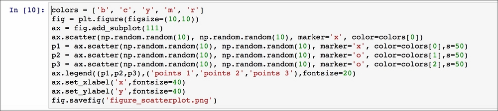
The s option represents the size of the points and colors are the colors that correspond to each set of points and the handles are passed directly into the legend function (p1, p2, p3):

Scatter plot of randomly distributed points
For further details on how to use matplotlib we advise the reader to read online material and tutorials such as http://matplotlib.org/users/pyplot_tutorial.html.