This algorithm is used to find the maximum likelihood estimates of parameter distribution models that depend on hidden (unobserved) variables. Expectation maximization consists of iterating two steps: the E-step, which creates the log-likelihood function evaluated using the current values of the parameters, and the M-step, where the new parameters' values are computed, maximizing the log-likelihood of the E-step.

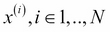
Consider a set of N elements, {x⁽ⁱ⁾}i = 1,…,N, and a log-likelihood on the data as follows:

Here, θ represents the set of parameters and z⁽ⁱ⁾ are the so-called hidden variables.

We want to find the values of the parameters that maximize the log-likelihood without knowing the values of the z⁽ⁱ⁾ (unobserved variables). Consider a distribution over the z⁽ⁱ⁾, and Q(z⁽ⁱ⁾), such as . Therefore:

This means Q(z⁽ⁱ⁾) is the posterior distribution of the hidden variable, z⁽ⁱ⁾, given x⁽ⁱ⁾ parameterized by θ. The expectation maximization algorithm comes from the use of Jensen's inequality and it ensures that carrying out these two steps:

The log-likelihood converges to the maximum, and so the associated θ values are found.

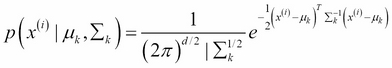
This method models the entire dataset using a mixture of Gaussian distributions. Therefore, the number of clusters will be given as the number of Gaussians considered in the mixture. Given a dataset of N elements, {x⁽ⁱ⁾}i = 1,…,N, where each is a vector of d-features modeled by a mixture of Gaussian such as the following:

Where:

The parameters of our model are thus φ, µ and ∑. To estimate them, we can write down the log-likelihood of the dataset:

In order to find the values of the parameters, we apply the expectation maximization algorithm explained in the previous section where and .

After choosing a first guess of the parameters, we iterate the following steps until convergence:

Note that the expectation maximization algorithm is needed because the hidden variables z⁽ⁱ⁾ are unknown. Otherwise, it would have been a supervised learning problem, where z⁽ⁱ⁾ is the label of each point of the training set (and the supervised algorithm used would be the Gaussian discriminant analysis). Therefore, this is an unsupervised algorithm and the goal is also to find z⁽ⁱ⁾, that is, which of the K Gaussian components each point x⁽ⁱ⁾ is associated with. In fact, by calculating the posterior probability for each of the K classes, it is possible to assign each x(i) to the class k with the highest posterior probability. There are several cases in which this algorithm can be successfully used to cluster (label) the data.

A possible practical example is the case of a professor with student grades for two different classes but not labeled per class. He wants to split the grades into the original two classes assuming that the distribution of grades in each class is Gaussian. Another example solvable with the mixture of the Gaussian approach is to determine the country of each person based on a set of people's height values coming from two different countries and assuming that the distribution of height in each country follows Gaussian distribution.

This algorithm tries to find the center of each cluster as the mean of all the members that minimize the distance between the center and the assigned points themselves. It can be associated with the k-nearest-neighbor algorithm in classification problems, and the resulting set of clusters can be represented as a Voronoi diagram (a method of partitioning the space in regions based on the distance from a set of points, in this case, the clusters' centers). Consider the usual dataset, . The algorithm prescribes to choose a number of centers K, assign the initial mean cluster centers to random values, and then iterate the following steps until convergence:

It decreases monotonically with the number of iterations. Since F is a nonconvex function, it is not guaranteed that the final minimum will be the global minimum. In order to avoid the problem of a clustering result associated with the local minima, the k-means algorithm is usually run multiple times with different random initial center's means. Then the result associated with the lower F value is chosen as the optimal clustering solution.

Mean-shift is nonparametric algorithm that finds the positions of the local maxima in a density kernel function defined on a dataset. The local maxima found can be considered the centers of clusters in a dataset , and the number of maxima is the number of clusters. In order to be applied as a clustering algorithm, each point has to be associated with the density of its neighborhood:

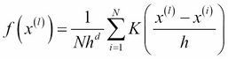
Here, h is the so-called bandwidth; it estimates the radius of the neighborhood in which the points affect the density value f(x^(l)) (that is, the other points have negligible effect on ). K is the kernel function that satisfies these conditions:

Typical examples of K(x⁽ⁱ⁾) are the following functions:

The mean-shift algorithm imposes the maximization of f(x^(l)), which translates into the mathematical equation (remember that in function analysis, the maximum is found by imposing the derivative to 0):

Here, K' is derivative of the kernel density function K.

Therefore, to find the local maxima position associated with the feature vector x^(l), the following iterative equation can be computed:

Here, is called the mean-shift vector. The algorithm will converge when at iteration t=a, the condition is satisfied.

Supported by the equation, we can now explain the algorithm with the help of the following figure. At the first iteration t=0, the original points (red) are spread on the data space, the mean shift vector is calculated, and the same points are marked with a cross (x) to track their evolution with the algorithm. At iteration 1, the dataset will be obtained using the aforementioned equation, and the resulting points are shown in the following figure with the (+) symbol:

Sketch of the mean-shift evolution through iterations

In the preceding figure, at iteration 0 the original points are shown in red (cross), at iteration 1 and K the sample points (symbols + and * respectively) move towards the local density maxima indicated by blue squares.

Again, at iteration K, the new data points are computed and they are shown with the * symbol in the preceding figure. The density function values associated with are larger than the values in the previous iterations since the algorithm aims to maximize them. The original dataset is now clearly associated with points , and they converge to the locations plotted in blue squares in the preceding figure. The feature vectors are now collapsing to two different local maxima, which represent the centers of the two clusters.

In order to properly use the method, some considerations are necessary.

The only parameter required, the bandwidth h, needs to be tuned cleverly to achieve good results. In fact, too low value of h may result in a large number of clusters, while a large value of h may merge multiple distinct clusters. Note also that if the number d of feature vector dimensions is large, the mean-shift method may lead to poor results. This is because in a very-high-dimensional space, the number of local maxima is accordingly large and the iterative equation can easily converge too soon.

To compare the clustering methods just presented, we need to generate a dataset. We choose the two dataset classes given by the two two-dimensional multivariate normal distributions with means and covariance equal to and , respectively.

The data points are generated using the NumPy library and plotted with matplotlib:

from matplotlib import pyplot as plt
import numpy as np
np.random.seed(4711)  # for repeatability 
c1 = np.random.multivariate_normal([10, 0], [[3, 1], [1, 4]], size=[100,])
l1 = np.zeros(100)
l2 = np.ones(100)
c2 = np.random.multivariate_normal([0, 10], [[3, 1], [1, 4]], size=[100,])
#add noise:
np.random.seed(1)  # for repeatability 
noise1x = np.random.normal(0,2,100)
noise1y = np.random.normal(0,8,100)
noise2 = np.random.normal(0,8,100)
c1[:,0] += noise1x
c1[:,1] += noise1y
c2[:,1] += noise2

fig = plt.figure(figsize=(20,15))
ax = fig.add_subplot(111)
ax.set_xlabel('x',fontsize=30)
ax.set_ylabel('y',fontsize=30)
fig.suptitle('classes',fontsize=30)
labels = np.concatenate((l1,l2),)
X = np.concatenate((c1, c2),)
pp1= ax.scatter(c1[:,0], c1[:,1],cmap='prism',s=50,color='r')
pp2= ax.scatter(c2[:,0], c2[:,1],cmap='prism',s=50,color='g')
ax.legend((pp1,pp2),('class 1', 'class2'),fontsize=35)
fig.savefig('classes.png')

A normally distributed noise has been added to both classes to make the example more realistic. The result is shown in the following figure:

Two multivariate normal classes with noise

The clustering methods have been implemented using the sklearn and scipy libraries and again plotted with matplotlib:

import numpy as np
from sklearn import mixture
from scipy.cluster.hierarchy import linkage
from scipy.cluster.hierarchy import fcluster
from sklearn.cluster import KMeans
from sklearn.cluster import MeanShift
from matplotlib import pyplot as plt

fig.clf()#reset plt
fig, ((axis1, axis2), (axis3, axis4)) = plt.subplots(2, 2, sharex='col', sharey='row')

#k-means
kmeans = KMeans(n_clusters=2)
kmeans.fit(X)
pred_kmeans = kmeans.labels_
plt.scatter(X[:,0], X[:,1], c=kmeans.labels_, cmap='prism')  # plot points with cluster dependent colors
axis1.scatter(X[:,0], X[:,1], c=kmeans.labels_, cmap='prism')
axis1.set_ylabel('y',fontsize=40)
axis1.set_title('k-means',fontsize=20)

#mean-shift
ms = MeanShift(bandwidth=7)
ms.fit(X)
pred_ms = ms.labels_
axis2.scatter(X[:,0], X[:,1], c=pred_ms, cmap='prism')
axis2.set_title('mean-shift',fontsize=20)

#gaussian mixture
g = mixture.GMM(n_components=2)
g.fit(X) 
pred_gmm = g.predict(X)
axis3.scatter(X[:,0], X[:,1], c=pred_gmm, cmap='prism')
axis3.set_xlabel('x',fontsize=40)
axis3.set_ylabel('y',fontsize=40)
axis3.set_title('gaussian mixture',fontsize=20)

#hierarchical
# generate the linkage matrix
Z = linkage(X, 'ward')
max_d = 110
pred_h = fcluster(Z, max_d, criterion='distance')
axis4.scatter(X[:,0], X[:,1], c=pred_h, cmap='prism')
axis4.set_xlabel('x',fontsize=40)
axis4.set_title('hierarchical ward',fontsize=20)
fig.set_size_inches(18.5,10.5)
fig.savefig('comp_clustering.png', dpi=100)

The k-means function and Gaussian mixture model have a specified number of clusters (n_clusters =2,n_components=2), while the mean-shift algorithm has the bandwidth value bandwidth=7. The hierarchical algorithm is implemented using the ward linkage and the maximum (ward) distance, max_d, is set to 110 to stop the hierarchy. The fcluster function is used to obtain the predicted class for each data point. The predicted classes for the k-means and the mean-shift method are accessed using the labels_ attribute, while the Gaussian mixture model needs to employ the predict function. The k -means, mean-shift, and Gaussian mixture methods have been trained using the fit function, while the hierarchical method has been trained using the linkage function. The output of the preceding code is shown in the following figure:

IClustering of the two multivariate classes using k-means, mean-shift, Gaussian mixture model, and hierarchical ward method

The mean-shift and hierarchical methods show two classes, so the choice of parameters (bandwidth and maximum distance) is appropriate. Note that the maximum distance value for the hierarchical method has been chosen looking at the dendrogram (the following figure) generated by the following code:

from scipy.cluster.hierarchy import dendrogram
fig = plt.figure(figsize=(20,15))
plt.title('Hierarchical Clustering Dendrogram',fontsize=30)
plt.xlabel('data point index (or cluster index)',fontsize=30)
plt.ylabel('distance (ward)',fontsize=30)
dendrogram(
    Z,
    truncate_mode='lastp',  # show only the last p merged clusters
    p=12,
    leaf_rotation=90.,
    leaf_font_size=12.,
    show_contracted=True,
)
fig.savefig('dendrogram.png')

The truncate_mode='lastp' flag allows us to specify the number of last merges to show in the plot (in this case, p=12). The preceding figure clearly shows that when the distance is between 100 and 135, there are only two clusters left:

IHierarchical clustering dendrogram for the last 12 merges

In the preceding figure on the horizontal axis, the number of data points belonging to each cluster before the last 12 merges is shown in brackets ().

Apart from the Gaussian mixture model, the other three algorithms misclassify some data points, especially k-means and hierarchical methods. This result proves that the Gaussian mixture model is the most robust method, as expected, since the dataset comes from the same distribution assumption. To evaluate the quality of the clustering, scikit-learn provides methods to quantify the correctness of the partitions: v-measure, completeness, and homogeneity. These methods require the real value of the class for each data point, so they are referred to as external validation procedures. This is because they require additional information not used while applying the clustering methods. Homogeneity, h, is a score between 0 and 1 that measures whether each cluster contains only elements of a single class. Completeness, c, quantifies with a score between 0 and 1 whether all the elements of a class are assigned to the same cluster. Consider a clustering that assigns each data point to a different cluster. In this way, each cluster will contains only one class and the homogeneity is 1, but unless each class contains only one element, the completeness is very low because the class elements are spread around many clusters. Vice versa, if a clustering results in assigning all the data points of multiple classes to the same cluster, certainly the completeness is 1 but homogeneity is poor. These two scores have a similar formula, as follows:

Here:

The v-measure is simply the harmonic mean of the homogeneity and the completeness:

These measures require the true labels to evaluate the quality of the clustering, and often this is not real-case scenario. Another method only employs data from the clustering itself, called silhouette, which calculates the similarities of each data point with the members of the cluster it belongs to and with the members of the other clusters. If on average each point is more similar to the points of its own cluster than the rest of the points, then the clusters are well defined and the score is close to 1 (it is close to -1, otherwise). For the formula, consider each point i and the following quantities:

The silhouette can be defined as

, and the silhouette score is the average of s(i) for all data points.

The four clustering algorithms we covered are associated with the following values of these four measures calculated using sklearn (scikit-learn):

from sklearn.metrics import homogeneity_completeness_v_measure
from sklearn.metrics import silhouette_score
res = homogeneity_completeness_v_measure(labels,pred_kmeans)
print 'kmeans measures, homogeneity:',res[0],' completeness:',res[1],' v-measure:',res[2],' silhouette score:',silhouette_score(X,pred_kmeans)
res = homogeneity_completeness_v_measure(labels,pred_ms)
print 'mean-shift measures, homogeneity:',res[0],' completeness:',res[1],' v-measure:',res[2],' silhouette score:',silhouette_score(X,pred_ms)
res = homogeneity_completeness_v_measure(labels,pred_gmm)
print 'gaussian mixture model measures, homogeneity:',res[0],' completeness:',res[1],' v-measure:',res[2],' silhouette score:',silhouette_score(X,pred_gmm)
res = homogeneity_completeness_v_measure(labels,pred_h)
print 'hierarchical (ward) measures, homogeneity:',res[0],' completeness:',res[1],' v-measure:',res[2],' silhouette score:',silhouette_score(X,pred_h)
The preceding code produces the following output:
kmeans measures, homogeneity: 0.25910415428  completeness: 0.259403626429  v-measure: 0.259253803872  silhouette score: 0.409469791511
mean-shift measures, homogeneity: 0.657373750073  completeness: 0.662158204648  v-measure: 0.65975730345  silhouette score: 0.40117810244
gaussian mixture model measures, homogeneity: 0.959531296098  completeness: 0.959600517797  v-measure: 0.959565905699  silhouette score: 0.380255218681
hierarchical (ward) measures, homogeneity: 0.302367273976  completeness: 0.359334499592  v-measure: 0.32839867574  silhouette score: 0.356446705251

As expected from the analysis of the preceding figure, the Gaussian mixture model has the best values of the homogeneity, completeness, and v-measure measures (close to 1); mean-shift has reasonable values (around 0.5); while k-means and hierarchical methods result in poor values (around 0.3). The silhouette score instead is decent for all the methods (between 0.35 and 0.41), meaning that the clusters are reasonably well defined.