
The generalized linear model is a group of models that try to find the M parameters ![]() that form a linear relationship between the labels yi and the feature vector x(i) that is as follows:
that form a linear relationship between the labels yi and the feature vector x(i) that is as follows:

Here, ![]() are the errors of the model. The algorithm for finding the parameters tries to minimize the total error of the model defined by the cost function J:
are the errors of the model. The algorithm for finding the parameters tries to minimize the total error of the model defined by the cost function J:

The minimization of J is achieved using an iterative algorithm called batch gradient descent:

Here, α is called learning rate, and it is a trade-off between convergence speed and convergence precision. An alternative algorithm that is called stochastic gradient descent, that is loop for ![]() :
:

The θj is updated for each training example i instead of waiting to sum over the entire training set. The last algorithm converges near the minimum of J, typically faster than batch gradient descent, but the final solution may oscillate around the real values of the parameters. The following paragraphs describe the most common model ![]() and the corresponding cost function, J.
and the corresponding cost function, J.
Linear regression is the simplest algorithm and is based on the model:

The cost function and update rule are:

Ridge regression, also known as Tikhonov regularization, adds a term to the cost function J such that:

![]() , where λ is the regularization parameter. The additional term has the function needed to prefer a certain set of parameters over all the possible solutions penalizing all the parameters θj different from 0. The final set of θjshrank around 0, lowering the variance of the parameters but introducing a bias error. Indicating with the superscript l the parameters from the linear regression, the ridge regression parameters are related by the following formula:
, where λ is the regularization parameter. The additional term has the function needed to prefer a certain set of parameters over all the possible solutions penalizing all the parameters θj different from 0. The final set of θjshrank around 0, lowering the variance of the parameters but introducing a bias error. Indicating with the superscript l the parameters from the linear regression, the ridge regression parameters are related by the following formula:

This clearly shows that the larger the λ value, the more the ridge parameters are shrunk around 0.
Lasso regression is an algorithm similar to ridge regression, the only difference being that the regularization term is the sum of the absolute values of the parameters:

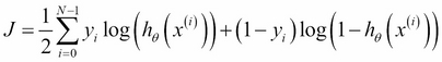
Despite the name, this algorithm is used for (binary) classification problems, so we define the labels![]() . The model is given the so-called logistic function expressed by:
. The model is given the so-called logistic function expressed by:

In this case, the cost function is defined as follows:
From this, the update rule is formally the same as linear regression (but the model definition, ![]() , is different):
, is different):

Note that the prediction for a point p, ![]() , is a continuous value between 0 and 1. So usually, to estimate the class label, we have a threshold at
, is a continuous value between 0 and 1. So usually, to estimate the class label, we have a threshold at ![]() =0.5 such that:
=0.5 such that:

The logistic regression algorithm is applicable to multiple label problems using the techniques one versus all or one versus one. Using the first method, a problem with K classes is solved by training K logistic regression models, each one assuming the labels of the considered class j as +1 and all the rest as 0. The second approach consists of training a model for each pair of labels ( trained models).
Now that we have seen the generalized linear model, let's find the parameters θj that satisfy the relationship:

In the case of linear regression, we can assume ![]() as normally distributed with mean 0 and variance σ2 such that the probability is
as normally distributed with mean 0 and variance σ2 such that the probability is  equivalent to:

Therefore, the total likelihood of the system can be expressed as follows:

In the case of the logistic regression algorithm, we are assuming that the logistic function itself is the probability:
Then the likelihood can be expressed by:

In both cases, it can be shown that maximizing the likelihood is equivalent to minimizing the cost function, so the gradient descent will be the same.
This is a very simple classification (or regression) method in which given a set of feature vectors ![]() with corresponding labels yi, a test point x(t) is assigned to the label value with the majority of the label occurrences in the K nearest neighbors
with corresponding labels yi, a test point x(t) is assigned to the label value with the majority of the label occurrences in the K nearest neighbors ![]() found, using a distance measure such as the following:
found, using a distance measure such as the following:
- Euclidean:

- Manhattan:

- Minkowski:
 (if q=2, this reduces to the Euclidean distance)
In the case of regression, the value yt is calculated by replacing the majority of occurrences by the average of the labels ![]()
![]() . The simplest average (or the majority of occurrences) has uniform weights, so each point has the same importance regardless of their actual distance from x(t). However, a weighted average with weights equal to the inverse distance from x(t) may be used.
. The simplest average (or the majority of occurrences) has uniform weights, so each point has the same importance regardless of their actual distance from x(t). However, a weighted average with weights equal to the inverse distance from x(t) may be used.