Naive Bayes is a classification algorithm based on Bayes' probability theorem and conditional independence hypothesis on the features. Given a set of m features, , and a set of labels (classes) , the probability of having label c (also given the feature set x_i) is expressed by Bayes' theorem:

Here:

The predicted class associated with the set of features will be the value p such that the probability is maximized:

However, the equation cannot be computed. So, an assumption is needed.

Using the rule on conditional probability , we can write the numerator of the previous formula as follows:

We now use the assumption that each feature x_i is conditionally independent given c (for example, to calculate the probability of x₁ given c, the knowledge of the label c makes the knowledge of the other feature x₀ redundant, ):

Under this assumption, the probability of having label c is then equal to:

––––––––(1)

Here, the +1 in the numerator and the M in the denominator are constants, useful for avoiding the 0/0 situation (Laplace smoothing).

Due to the fact that the denominator of (1) does not depend on the labels (it is summed over all possible labels), the final predicted label p is obtained by finding the maximum of the numerator of (1):

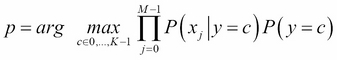––––––––(2)

Given the usual training set , where (M features) corresponding to the labels set , the probability P(y=c) is simply calculated in frequency terms as the number of training examples associated with the class c over the total number of examples, . The conditional probabilities instead are evaluated by following a distribution. We are going to discuss two models, Multinomial Naive Bayes and Gaussian Naive Bayes.

Multinomial Naive Bayes

Let's assume we want to determine whether an e-mail s given by a set of word occurrences is spam (1) or not (0) so that . M is the size of the vocabulary (number of features). There are words and N training examples (e-mails).

Each email x⁽ⁱ⁾ with label y_i such that is the number of times the word j in the vocabulary occurs in the training example l. For example, represents the number of times the word 1, or w₁, occurs in the third e-mail. In this case, multinomial distribution on the likelihood is applied:

Here, the normalization constants in the front can be discarded because they do not depend on the label y, and so the arg max operator will not be affected. The important part is the evaluation of the single word w_j: probability over the training set:

Here N_iy is the number of times the word j occurs, that is associated with label y, and N_y is the portion of the training set with label y.

This is the analogue of , on equation (1) and the multinomial distribution likelihood. Due to the exponent on the probability, usually the logarithm is applied to compute the final algorithm (2):

Gaussian Naive Bayes

If the features vectors x⁽ⁱ⁾ have continuous values, this method can be applied. For example, we want to classify images in K classes, each feature j is a pixel, and x_j⁽ⁱ⁾ is the j-th pixel of the i-th image in the training set with N images and labels . Given an unlabeled image represented by the pixels , in this case, in equation (1) becomes:

Here:

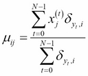
And: