
Although this method cannot be strictly considered a supervised learning algorithm, it can be also used to perform something that is really similar to classification, so we decided to include it here. To introduce the subject, we are going to present an example. Consider the simplistic case of predicting whether a salesman in front of you is lying or not (two states ![]() ) by observing his glance: eye contact, looking down, or looking aside (each observation Oi has the values 0, 1, and 2 respectively). Imagine a sequence of observations of the salesman's glances O=O0, O1, O2, O3, O4,… are 0, 1, 0, 2,… We want to infer the transition matrix A between states Si at consecutive times t, t+1 (or, in this example, two consecutive sentences):
) by observing his glance: eye contact, looking down, or looking aside (each observation Oi has the values 0, 1, and 2 respectively). Imagine a sequence of observations of the salesman's glances O=O0, O1, O2, O3, O4,… are 0, 1, 0, 2,… We want to infer the transition matrix A between states Si at consecutive times t, t+1 (or, in this example, two consecutive sentences):

Any entry of A, aij represents the probability to stay at state Si at time t+1 given the state Sj at time t. Therefore, 0.3 (a01) is the probability that the salesman is not lying on the sentence at time t+1 given that he is lying on the sentence at time t, 0.6 (a10) is vice versa, 0.7(a00) represents the probability that the salesman is lying on the sentence at time t and at time t+10.4(a11) is the probability that he is not lying on the sentence at time t+1 after he was sincere at time t. In a similar way, it is possible to define the matrix B that correlates the salesman's intention with his three possible behaviors:

Any entry bj(k) is the probability to have observation k at time t given the state Sj at time t. For example, 0.7 (b00), 0.1 (b01), and 0.2 (b02) are the probabilities that the salesman is lying given the behavioral observations—eye contact, looking down, and looking aside—respectively. These relationships are described in the following figure:

Salesman behavior – two states hidden Markov model
The initial state distribution of the salesman can be also defined: ![]() (he is slightly more inclined to lie than to tell the truth in the first sentence at time 0). Note that all of these matrices
(he is slightly more inclined to lie than to tell the truth in the first sentence at time 0). Note that all of these matrices ![]() are row stochastic; that is, the rows sum to 1 and there is no direct dependency on time. A hidden Markov model (HMM) is given by the composition of the three matrices (
are row stochastic; that is, the rows sum to 1 and there is no direct dependency on time. A hidden Markov model (HMM) is given by the composition of the three matrices (![]() ) that describe the relationship between the known sequence of observations O=O0, O1,…OT-1 and the corresponding hidden states sequence S=S0, S1,… ST-1. In general, the standard notation symbols employed by this algorithm are summarized as follows:
) that describe the relationship between the known sequence of observations O=O0, O1,…OT-1 and the corresponding hidden states sequence S=S0, S1,… ST-1. In general, the standard notation symbols employed by this algorithm are summarized as follows:
- T is the length of the observation sequence O=O0, O1,… OT-1 and the hidden states sequence S=S0, S1,… ST-1
- N is the number of possible (hidden) states in the model
- M is the number of the possible observation values:

- A is the state transition matrix
- B is the observation probability matrix
- π is the initial state distribution
In the preceding example, M=3, N=2, and we imagine to predict the sequence of the salesman's intentions over the course of his speech (which are the hidden states) S=S0, S1,… ST-1, observing the values of his behavior O=O0, O1,… OT-1. This is achieved by calculating the probability of each state sequence S as:
For instance, fixing T=4, S=0101, and O=1012:
In the same way, we can calculate the probability of all other combinations of hidden states and find the most probable sequence S. An efficient algorithm for finding the most probable sequence S is the Viterbi algorithm, which consists of computing the maximum probability of the set of partial sequences from 0 to t until T-1. In practice, we calculate the following quantities:

-
For t=1,…,T-1 and i=0,…,N-1, the maximum probability of being at state i at time t among the possible paths coming from different states j is
 . The partial sequence associated with the maximum of
  is the most probable partial sequence until time t.
-
The final most probable sequence is associated with the maximum of the probability at time T-1:
 .
.
For example, given the preceding model, the most likely sequence of length T=2 can be calculated as:
- P(10)=0.0024
- P(00)=0.0294
- So d1(0)=P(00)=0.0294
- P(01)=0.076
- P(11)=0.01
- So d1(1)=P(01)=0.076
And the final most probable sequence is 00 (two consecutive false sentences).
Another way to think about the most likely sequence is by maximizing the number of correct states; that is, consider for each time t the state i with the maximum probability ![]() . Using an algorithm called backward algorithm, it is possible to show that the probability of a given state i,
. Using an algorithm called backward algorithm, it is possible to show that the probability of a given state i, ![]() , is:
, is:

Here:

 and
and  Probabilities of the partial observation sequence until time t, where the HMM is on state i:
 and
and  Probability of the partial sequence after time t until T-1 given the state at time t equal to i:
-
The combination of the probabilities to stay on state i before and after time t result in the value of
 .
.
Note that the two methods of calculating the most likely sequence do not necessarily return the same result.
The reverse problem—find the optimal HMM ![]() given a sequence O=O0,O1,…OT-1 and the values of the parameters N, M—is also solvable iteratively using the
Baum-Welch algorithm. Defining the probability of occurring at state i at time t and to go at state j at time t+1 as:
given a sequence O=O0,O1,…OT-1 and the values of the parameters N, M—is also solvable iteratively using the
Baum-Welch algorithm. Defining the probability of occurring at state i at time t and to go at state j at time t+1 as:
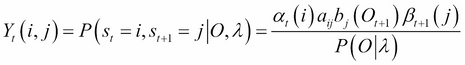 where
where  for
for ![]() and
and  .
.
Then the Baum-Welch algorithm is as follows:
-
Initialize

-
Calculate
 and
and 
- Recompute the model matrices as:
 where
where  and
and  is Kronacker symbol, which is equal to 1 if
  and 0 otherwise
-
Iterate until the convergence of:

In the next section, we are going to show a piece of Python code that implements these equations to test the HMM algorithm.
As usual, the hmm_example.py file discussed hereafter is available at https://github.com/ai2010/machine_learning_for_the_web/tree/master/chapter_3/.
We start defining a class in which we pass the model matrices:
class HMM:
    def __init__(self):

self.pi = pi
        self.A = A
        self.B = B
The Viterbi algorithm and the maximization of the number of correct states are implemented in the following two functions:
    def ViterbiSequence(self,observations):
        deltas = [{}]
        seq = {}
        N = self.A.shape[0]
        states = [i for i in range(N)]
        T = len(observations)
        #initialization
        for s in states:
            deltas[0][s] = self.pi[s]*self.B[s,observations[0]]
            seq[s] = [s]
        #compute Viterbi
        for t in range(1,T):
            deltas.append({})
            newseq = {}
            for s in states:
                (delta,state) = max((deltas[t-1][s0]*self.A[s0,s]*self.B[s,observations[t]],s0) for s0 in states)
                deltas[t][s] = delta
                newseq[s] = seq[state] + [s]
            seq = newseq

        (delta,state) = max((deltas[T-1][s],s) for s in states)
        return  delta,' sequence: ', seq[state]

    def maxProbSequence(self,observations):
        N = self.A.shape[0]
        states = [i for i in range(N)]
        T = len(observations)
        M = self.B.shape[1]
        # alpha_t(i) = P(O_1 O_2 ... O_t, q_t = S_i | hmm)
        # Initialize alpha
        alpha = np.zeros((N,T))
        c = np.zeros(T) #scale factors
        alpha[:,0] = pi.T * self.B[:,observations[0]]
        c[0] = 1.0/np.sum(alpha[:,0])
        alpha[:,0] = c[0] * alpha[:,0]
        # Update alpha for each observation step
        for t in range(1,T):
            alpha[:,t] = np.dot(alpha[:,t-1].T, self.A).T * self.B[:,observations[t]]
            c[t] = 1.0/np.sum(alpha[:,t])
            alpha[:,t] = c[t] * alpha[:,t]

        # beta_t(i) = P(O_t+1 O_t+2 ... O_T | q_t = S_i , hmm)
        # Initialize beta
        beta = np.zeros((N,T))
        beta[:,T-1] = 1
        beta[:,T-1] = c[T-1] * beta[:,T-1]
        # Update beta backwards froT end of sequence
        for t in range(len(observations)-1,0,-1):
            beta[:,t-1] = np.dot(self.A, (self.B[:,observations[t]] * beta[:,t]))
            beta[:,t-1] = c[t-1] * beta[:,t-1]

        norm = np.sum(alpha[:,T-1])
        seq = ''
        for t in range(T):
            g,state = max(((beta[i,t]*alpha[i,t])/norm,i) for i in states)
            seq +=str(state)

        return seq
Since the multiplication of probabilities will result in an underflow problem, all the Αt(i) and Βt(i) have been multiplied by a constant such that for ![]() :
:

 where
where 
Now we can initialize the HMM model with the matrices in the salesman's intentions example and use the two preceding functions:
pi = np.array([0.6, 0.4])
A = np.array([[0.7, 0.3],
                           [0.6, 0.4]])
B = np.array([[0.7, 0.1, 0.2],
                           [0.1, 0.6, 0.3]])
hmmguess = HMM(pi,A,B)
print 'Viterbi sequence:',hmmguess.ViterbiSequence(np.array([0,1,0,2]))
print 'max prob sequence:',hmmguess.maxProbSequence(np.array([0,1,0,2]))
The result is:
Viterbi: (0.0044, 'sequence: ', [0, 1, 0, 0])
Max prob sequence: 0100
In this particular case, the two methods return the same sequence, and you can easily verify that by changing the initial matrices, the algorithms may lead to different results. We obtain that the sequence of behaviors; eye contact, looking down, eye contact, looking aside is likely associated with the salesman states' sequence; lie, not lie, lie, lie with a probability of 0.0044.
It is also possible to implement the Baum-Welch algorithm to find the optimal HMM given the sequence of observations and the parameters N and M. Here is the code:
    def train(self,observations,criterion):

        N = self.A.shape[0]
        T = len(observations)
        M = self.B.shape[1]

        A = self.A
        B = self.B
        pi = copy(self.pi)

        convergence = False
        while not convergence:

            # alpha_t(i) = P(O_1 O_2 ... O_t, q_t = S_i | hmm)
            # Initialize alpha
            alpha = np.zeros((N,T))
            c = np.zeros(T) #scale factors
            alpha[:,0] = pi.T * self.B[:,observations[0]]
            c[0] = 1.0/np.sum(alpha[:,0])
            alpha[:,0] = c[0] * alpha[:,0]
            # Update alpha for each observation step
            for t in range(1,T):
                alpha[:,t] = np.dot(alpha[:,t-1].T, self.A).T * self.B[:,observations[t]]
                c[t] = 1.0/np.sum(alpha[:,t])
                alpha[:,t] = c[t] * alpha[:,t]

            #P(O=O_0,O_1,...,O_T-1 | hmm)
            P_O = np.sum(alpha[:,T-1])
            # beta_t(i) = P(O_t+1 O_t+2 ... O_T | q_t = S_i , hmm)
            # Initialize beta
            beta = np.zeros((N,T))
            beta[:,T-1] = 1
            beta[:,T-1] = c[T-1] * beta[:,T-1]
            # Update beta backwards froT end of sequence
            for t in range(len(observations)-1,0,-1):
                beta[:,t-1] = np.dot(self.A, (self.B[:,observations[t]] * beta[:,t]))
                beta[:,t-1] = c[t-1] * beta[:,t-1]

            gi = np.zeros((N,N,T-1));

            for t in range(T-1):
                for i in range(N):

                    gamma_num = alpha[i,t] * self.A[i,:] * self.B[:,observations[t+1]].T *
                            beta[:,t+1].T
                    gi[i,:,t] = gamma_num / P_O

            # gamma_t(i) = P(q_t = S_i | O, hmm)
            gamma = np.squeeze(np.sum(gi,axis=1))
            # Need final gamma element for new B
            prod =  (alpha[:,T-1] * beta[:,T-1]).reshape((-1,1))
            gamma_T = prod/P_O
            gamma = np.hstack((gamma,  gamma_T)) #append one Tore to gamma!!!

            newpi = gamma[:,0]
            newA = np.sum(gi,2) / np.sum(gamma[:,:-1],axis=1).reshape((-1,1))
            newB = copy(B)

            sumgamma = np.sum(gamma,axis=1)
            for ob_k in range(M):
                list_k = observations == ob_k
                newB[:,ob_k] = np.sum(gamma[:,list_k],axis=1) / sumgamma

            if np.max(abs(pi - newpi)) < criterion and
                   np.max(abs(A - newA)) < criterion and
                   np.max(abs(B - newB)) < criterion:
                convergence = True;

            A[:],B[:],pi[:] = newA,newB,newpi

        self.A[:] = newA
        self.B[:] = newB
        self.pi[:] = newpi
        self.gamma = gamma
Note that the code uses the shallow copy from the module copy, which creates a new container populated with references to the contents of the original object (in this case, pi, B). That is, newpi is a different object from pi but newpi[0] is a reference of pi[0]. The NumPy squeeze function instead is needed to drop the redundant dimension from a matrix.
Using the same behaviors sequence O=0, 1, 0, 2, we obtain that the optimal model is given by:
![]() ,
, ,
,
This means that the state sequence must start from a true salesman's sentence and continuously oscillate between the two states lie and not lie. A true salesman's sentence (not lie) is certainly related to the eye contact value, while a lie is related to the looking down and looking aside behaviors.
In this simple introduction on HMM, we have assumed that each observation is a scalar value, but in real applications, each Oi is usually a vector of features. And usually, this method is used as a classification training as many HMM li, as classes to predict and then a test time chooses the class with the highest ![]() . Continuing with this example, we can imagine building a true machine to test each salesman we talk to. Imagine that for each sentence (observation) Oi of our speaker, we can extract three features glances with three possible values ei (eye contact, looking down, and looking aside), voice sound vi with three possible values (too loud, too low, and flat), and hand movement hi with two possible values (shaking and calm) Oi=(ei, vi, hi). At training time, we ask our friend to tell lies and we use these observations to train an HMM l0 using Baum-Welch. We repeat the training process but with true sentences and train l1. At test time, we record the sentence of the salesman O and calculate both:
. Continuing with this example, we can imagine building a true machine to test each salesman we talk to. Imagine that for each sentence (observation) Oi of our speaker, we can extract three features glances with three possible values ei (eye contact, looking down, and looking aside), voice sound vi with three possible values (too loud, too low, and flat), and hand movement hi with two possible values (shaking and calm) Oi=(ei, vi, hi). At training time, we ask our friend to tell lies and we use these observations to train an HMM l0 using Baum-Welch. We repeat the training process but with true sentences and train l1. At test time, we record the sentence of the salesman O and calculate both: ![]() ,
,![]() . The class prediction will be the one with the highest probability.
. The class prediction will be the one with the highest probability.
Note that HMM has been applied in various fields, but the applications in which it performs quite well are speech recognition tasks, handwritten character recognition, and action recognition.