
3
Complexity and Chaos
As far as the laws of mathematics refer to reality, they are not certain; as far as they are certain they do not refer to reality.
– Albert Einstein
Research in chaos is the most interesting current area that there is. I am convinced that chaos research will bring about a revolution in the natural sciences similar to that produced by quantum mechanics.
– Gerd Binnig, Nobel Prize winner in Physics (1986)
3.1. Introduction
Chaos science came to light in the mid-1970s and has had an impact on a host of scientific disciplines from theoretical physics to insurance, economics, meteorology and medicine. It throws doubt on our ability to predict future events accurately. In spite of advanced and costly marketing research, a large proportion of new product introductions turn out to be failures. It sounds as if we are doing no better than chance, or even worse. In fact, chaos science affects our daily life. It can help us to understand such phenomena as the spread of diseases, the stock market volatility, the lack of reliability of weather forecasts and product sales.
Chaos science is the popular name for the study of nonlinear dynamic systems. It has made scientists more aware of the fact that most quantitative models they design and use are linearized approximations of what they observe as reality. Among the new understandings are:
- – apparently simple systems can be quite complicated in their operations;
- – apparently complicated systems can be quite simple in their operations;
- – a system can be perfectly deterministic and yet its behavior impossible to predict.
In fact, the concept of chaos has already been apprehended in ancient Chinese, Greek and Roman civilizations.
In old Chinese traditional thinking, chaos and order are interrelated ideas. In Chinese mythology, the dragon symbolizes Yang, the active male principle of universe. It is the concept of order that proceeds from chaos. In some Chinese, stories of the creation, Yin, the passive female principle of universe, is viewed as a ray of light from chaos to create heavens. Yin and Yang, male and female ontological objects, respectively, co-create the universe. After having sprung from chaos, Yin and Yang retain stigmata of chaos. When one of them surpasses the other, chaos is brought back.
The Greek Hesiodus (8th Century BC) wrote a cosmologist composition in which he posited that chaos existed before all things and the earth, in other words, order comes from disorder. Nothing was deduced from this mythical idea until the 20th Century when the chaos theory emerged.
The term is defined by Virgil (Georgica IV, 347) as “a state of confusion having preceded the organization of the world”. It was figuratively used at the time of the lower Roman Empire (4th Century AD – Marcus Victorinus) and by the Fathers of the Church (4th Century AD) to characterize the state of the earth before God’s creative intervention. Chaos rendered the Hebrew word tohu-bohu.
Chaos is derived from Greek χαος referring in mythology to the early state of the universe before gods were born and also to the mindset of infinite space, abyss and chasm (in modern Greek). It is also connected to the German word Gaumen (mouth palate) in relationship with the Indo-European root ghen, which expresses vacuum and lack.
Chaos conveys the idea of the state of confusion of the elements before the world was organized in the Antique and Christian cosmologies. By extension, it suggests a state of great confusion with a specialized acceptation in politics (Voltaire, 1756) and in the concrete bears the meaning of heaps of rock blocks (1796).
In the 19th Century, the word chaos has gained in science a special value of “random distribution, without describable order, of positions and velocities of molecules” of perfect gases in equilibrium. From 1890 onwards, the adjective chaotic showed up with a strong or weakened meaning of “incoherence, disorder”.
Chaos has been instanced for a long time by gases, the construct model of which is made up of the erratic motions of particles. The word “gas” was introduced by the Dutch physician chemist van Helmont (1579–1644) from the Latin word chaos by changing “ch” to “g” according the pronunciation of “g” in Dutch.
When an observed phenomenon is qualified as chaotic by an observer, the question to investigate is: “is this phenomenon deterministically chaotic or the consequence of genuine randomness?” This is the core issue we shall address in this chapter.
3.2. Complexity and chaos in physics and chemistry
3.2.1. Introductory considerations
Physics is mainly concerned with abstracting simple concepts from a complex world. Newton found simple gravitation laws that could predict planetary motion on the basis of the attraction of two bodies. Results from atomic physics have demonstrated that the Schrödinger equation is the correct description of a hydrogen atom, composed of a positive nucleus and an orbiting negative electron.
A. M. Turing when presenting his model of the chemical basis of morphogenesis (Turing 1952) insisted on the very nature of a model: “this model will be a simplification and an idealization, and consequently a falsification. It is to be hoped that the features retained for discussion are those of greatest importance in the present state of knowledge.” WYSIATI (What You See Is All There Is) does not hold true. Simple models are substituted for encoding of physical laws. These models, when validated, yield the same predictions and results we observe. In some cases, we do not even know the exact equations governing the phenomena considered. These models have nothing to do with what happens at the micro-levels of phenomena.
When many-body systems are considered, the basic models are called upon to produce equations. In general, these equations have no analytical solutions. Physicists and chemists working in different disciplines have developed a variety of methods for obtaining approximate but reliable estimates of the properties and behaviors of many-body systems. These techniques are regarded as a “tool box” needed to tackle the many-body problems. They may be used to study any many-particle system for which the interactions are known.
In astronomy, the three-body problem of interacting planets in a gravitational field (for instance, the Sun, the Earth and the Moon) was studied by the mathematician Henri Poincaré at the turn of the 20th Century but an analytical solution was not delivered. Careful analysis shows that an unstable trajectory can develop under certain conditions of parameter values. This is a sign of possible chaos from a long-range point of view. Ahead of his time, almost 100 years ago, Henri Poincaré first suggested the notion of SDCI (sensitive dependence upon initial conditions).
“Much of chaos as science is connected to the notion of sensitive dependence on initial conditions. Technically, scientists term as chaotic those non-random complicated motions that exhibit a rapid growth of errors that despite perfect determinism inhibits any pragmatic ability to render accurate long-term prediction.” (Feigenbaum 1992).
The Russian-born Jewish physician Immanuel Velikovsky (1875–1979) investigated events related in the Bible. In his book Colliding Worlds (1948), he asserted that the orbits of Mars and Venus experience a drastic change about 1000 years BC. His theory helped to solve some problems in agreement with the chronology of the antique world.
If variables that complicate matters get in the way, they are generally dealt with by ignoring them or assuming that their effects are random and do not result from a determinist law. On average in the long term, they will cancel themselves out. Those who have taken a course in physics may well remember that most test problems ended with “ignore the effects of friction” or “assume that the wind resistance is zero”. In the real world, friction cannot be ignored and the wind blows from all directions. Most elementary physics textbooks describe a world that seems filled with very simple, regular and symmetrical systems. A student might get the impression that atomic physics is the hydrogen atom, electromagnetic phenomena appear more often in the world in guises like the parallel plate capacitor and regular crystalline solids are “typical” materials.
The reality is that linear relationships are actually the exception in the world rather than the rule. A book written by the physicist Carlo Rovelli (2017) has the telling title Reality Is Not What It Seems. It is critical to bear in mind that approximation of reality by simplified models is valid under certain conditions. When these conditions are no longer fulfilled, the models involved cannot be referred to for understanding observations. The way to deal with this type of situation is to distribute observations into different categories, each of them described by the same model.
Let us take the example of inorganic chemistry. Chemical reactions can be itemized by the observable differences in the ease with which reactions occur. The following are their descriptions:
- – type A. Reactions that occur very readily, as soon as the reagents are mixed. Reactions of this kind usually involve gases or solutions. In the case of a liquid reacting with a solid, the rate is limited only by the time taken for the reactants to meet and the products to break away;
- – type B. Reactions that readily proceed if they are started with application of heat, but that proceed very slowly or not at all when the reactants are mixed at room temperature. In some cases, instead of heat, a catalyst will start the reaction;
- – type C. Reactions that take in heat and are termed “endothermic”. In general, such reactions only continue if a high temperature is maintained by an external supply;
- – type D. Reactions that proceed slowly but steadily. The velocity of reaction is well defined as the decrease in the concentration of one reactant per unit of time;
- – type E. Reversible reactions: reactions that readily proceed under certain conditions, but reverse if the conditions are changed. A reaction that reaches equilibrium can be taken nearer to completion if one of the products is removed;
- – type F. Reactions that do not proceed at all, at any temperature, without an external supply of energy.
Another interesting example is the description of electrical properties of solid-state materials. They are categorized into three groups: conductors, semiconductors and isolators, each group being characterized by a specific model.
Furthermore, some models of what we call “reality” are dealt with in spaces different from the three-dimensional space we are used to perceiving around us. Two spaces are important: the phase space in classical physics and the Hilbert space in quantum physics. The phase space is constructed to “visualize” the evolution of a system of n particles. It has a large number of dimensions (three position coordinates and three momentum coordinates representing the location and motion of each particle). For n unconstrained particles, there will be a “space” of 6 n dimensions. A single point of a phase state represents the entire state of some physical system. In quantum theory, the appropriate corresponding concept is that of a Hilbert space. A single point of Hilbert space represents the quantum state of an entire system. The most fundamental property of a Hilbert space is that it is what is called a vector space, in fact a complex vector space. This means that any two elements of the space can be added to obtain another such element with complex-weightings. Complex refers here to complex numbers.
Before the advent of computers, it was difficult to numerically solve nonlinear equations. That is the reason why great efforts were made to find approximate linear relationships of nonlinear relationships. However, this search for the simple models makes our description of the world seem to be a caricature rather than a portrait.
Three basic questions for trying to understand the fabric of the laws we are confronted with as humans are:
- – how do simple laws give rise to richly intricate structures? Many examples of this can be found in natural sciences and economics.
- – why are such structures so ubiquitous in the observed world?
- – why is it that these structures often embody their own kind of simple laws?
Let us try to consider some facts and meaning in attempting to answer these questions. The symptom of WYSIATI (What You See Is All There Is) has become the syndrome of our addiction to resort only to our sense-data. When we cannot interpret and visualize what our brain has constructed from sense signals received, we are tempted to qualify the situation as “complex”. We depend upon the perceivable (measurable) variables from our senses or equipment made available. These variables are derived from statistical laws. The micro-causes of effects are hidden to our senses. Statistical laws are applicable to a large assembly of entities and describe it in static and dynamic quantities according to the context. When a variable appears stable, we are in fact perceiving an average value manifesting the behaviors of a large number of interacting entities. A statistical distribution is maintained because of the existence of interaction processes between these entities.
Chaos, short for deterministic chaos, is quite different from randomness in spite of the fact that it is what it looks like. Chaos is absolutely fundamental to differential equations (or difference equations when discrete time events are considered), and these are the basic material required to encode physical laws. The paramount consequence is that irregular behavior need not have irregular causes. Deterministic implies that knowledge of the present determines the future uniquely and exactly.
Models in classical physics are underpinned by two main principles: Newton’s law of motion and conservation of mass:
- – Newton’s law of motion states that the acceleration of a body is proportional to the forces that act on it, regardless of their very nature, gravitational or electromagnetic;
- – the principle of mass conservation, implicit in numerous models, states that the rate at which a substance increases or decreases within some closed environment must be due solely to the rate at which matter enters from the outside minus the rate at which it leaves. If there are sources or sinks of matter inside the closed environment, they have to be accounted for.
It is noteworthy that these principles deal with motion, i.e. variation of distance or physical quantity over time. This implies that models are embodied by differential equations with respect to time, Ẋ = F[X(t)], where X(t) represents all the time-dependent parameters characterizing the model under consideration and Ẋ is the derivative of X(t) with respect to time. Stability of solutions derived from differential equations is a central issue to address.
The question of stability is related to any equilibrium state ![]() Equilibrium states are also called fixed points or orbits when periodic motions occur.
Equilibrium states are also called fixed points or orbits when periodic motions occur. ![]() states are solutions of the equation
states are solutions of the equation ![]() The issue to address is: if a physical system initially at rest is perturbed, does it gradually return to the initial position or does it wander about or will it at least remain in the vicinity of the initial position when t →∞?
The issue to address is: if a physical system initially at rest is perturbed, does it gradually return to the initial position or does it wander about or will it at least remain in the vicinity of the initial position when t →∞?
If the physical system returns to the initial position ![]() , then it is said to be stable, otherwise it is unstable. Unstable equilibriums represent states that one is unlikely to observe physically. When the trajectory of points X(t) starts in a domain of initial values X(0) for which
, then it is said to be stable, otherwise it is unstable. Unstable equilibriums represent states that one is unlikely to observe physically. When the trajectory of points X(t) starts in a domain of initial values X(0) for which
![]() , then X is said to be asymptotically stable. The domain is called the basin of attraction of
, then X is said to be asymptotically stable. The domain is called the basin of attraction of ![]() , and
, and ![]() its attractor.
its attractor.
Several models are represented by nonlinear differential equations, which is common place in reality. In this case, how to investigate their stability at their equilibrium states? The answer is linearization. This means that the curve that represents the spatial unfolding of the time-dependent variables is substituted for its tangent at the fixed points and the local stability is analyzed on this basis. So to speak, linearization is a misleading rendering of reality, but is the only way we have found to easily come to terms with the complexity of reality.
In the next section, the behavior of a quadratic iterative function is described. It serves as a simple instance of deterministic chaos in many publications. It shows how one of the simplest equations, modeling a population of living creatures, can generate chaotic behavior.
3.2.2. Quadratic iterator modeling the dynamic behavior of animal and plant populations
One of the first to draw attention to the chaotic behavior of nonlinear difference equations was the Australian ecologist Robert May, when in 1975 he published a paper on modeling changes in plant and animal population in an ecosystem when there are limits to the available resources.
Letting time events t tick in integer steps, corresponding to generations, the incumbent population is measured as a fraction supposed to represent the ratio between a current value and an estimated maximum value. The equation states

It is called the logistic equation, which can be easily transformed in a difference equation.

The population should settle to a steady state when Xt+1 = Xt. This leads to two steady states: population 0 and (k − 1/k). A population of size 0 is extinct, so the other value applies to an existing situation.
This quadratic iterator, a simple feedback process, has been widely investigated (Feigenbaum 1992). Its behavior depends on the value of the parameter k. As a function of its value, a wide variety of behaviors can be observed. The mechanisms are made well observable by graphical iteration (Figure 3.1). Graphical iteration is represented by a path with horizontal and vertical steps, which is called a poly-line for convenience.

Figure 3.1. Graphical paths to derive the iterates step by step from the initial value X0
The parabola k X (1 − X) is the graph of the iteration function and is the locus of points (Xt,,Xt+1). The vertex of the parabola is defined by its coordinates (X = 0.5, k/4). The parabola intersects the bisector at the fixed points P0 = 0 and Pk = (k − 1)/k along the abscissa scale. Only the initial values X0 = 0 and X0 = 1 are attracted by P0.
We start with an initial value X0 along the abscissa scale. At this value point a perpendicular to the abscissa scale is erected until it intersects the parabola at the X1 point, whose ordinate value reads along the ordinate scale. Via the bisector, the X1 point is transferred to the abscissa scale and the same mechanism is iterated to yield the X2 point. This procedure is repeated until a stabilized situation is reached. By stabilized, it is meant that the procedure produces an equilibrium point or a well-defined periodic cycle of different states. In some situations, neither an equilibrium point nor a periodic cycle is observed. The behavior appears chaotic.
For each starting value, the number of steps required to reach a stable situation (rest point or cyclic loop) is computed and called a “time profile”.
When k < 1, all initial values converge to P0, which is a stable point. Any point initially derived from X0 = 0 by a small deviation ε is attracted back to P0.
When 1 < k < 2, all initial values X0 progress step by step to an equilibrium value which is at the intersection of the bisector and the parabola along the abscissa scale. In this situation, P0 (Xt = 0) is not a stable fixed point. When Xt = 0 → Xt+n = 0 + ε through some perturbation, Xt migrates step by step monotonically to the equilibrium value at the intersection of the bisector and the parabola. By monotonically, it is meant that the approach to the equilibrium value takes place by either decreasing or increasing values without oscillations.
When 2 < k < 3, all initial values X0 progress step by step through a poly-line of damped oscillations to an equilibrium value, which is at the intersection of the bisector and the parabola along the abscissa scale. By damped oscillations, it is meant that the equilibrium value is alternatively approached by higher and lower values whose amplitudes decrease.
The fixed point Pk is the attractor of all poly-lines when 1< k<3.
When k = 3, a new regime under which the system operates emerges. Disruption of a sort appears. Even if a steady state is computationally expected, i.e. the equilibrium point at the intersection of the bisector and the parabola, it is never reached. Pk still exists. It has turned out to be an unstable repeller when k has crossed the border line k = 3, and as such cannot be observed.
What is observed is a stabilizing loop oscillating between two values, a lower one XL(k) and a higher one XH(k). This phenomenon is called “bifurcation”, and this point is called a bifurcation point.
The graphical analysis of iterated f(X) = k X (1 − X) appears clearly inadequate to explain the bifurcation phenomenon. It is necessary to find another function, which has the same characteristics in terms of time profiles, poly-line paths and fixed points. The function f [f(X)] fulfils these requirements. It is the first iterate of f(X). F(X) is then labeled f0(X) and f [f(X)] is labeled
f1(X).
The graph of f1(X) is given by the fourth-degree polynomial

It can be proved that this polynomial has four fixed points (intersection with the bisector), X = 0, X = (k − 1)/k, X = (k + 1)/2k ± √(k2 − 2k − 3)/4k2
X = 0 and X = (k − 1)/k are fixed points common with f0(X). The stabilized state is a cycle of period two oscillating between

and XH(k) = (k + 1)/2k + √[(k2 − 2k − 3)/4k2]
As k increases, other bifurcation points manifest themselves with period-doubling cycles (4, 8, 16, 32, etc.) each time. For instance, when 3.05 < k < 3.5, a bifurcation point is observed with a period-doubling cycle of four values.
The distance between two successive parameter k values of bifurcation points, dn = (kn+1 − kn), rapidly decreases when n increases. Observations show that the decrease in dn from bifurcation to bifurcation is approximately geometric, so that δn = dn/dn+1 is assumed to converge to δ when n → ∞. Feigenbaum (1975) calculated the value of this parameter, 4.669201, for the quadratic iterator. Investigations revealed that δ has the same value for a wide range of quadratic-like iterators. The value 4.669201 is now called the Feigenbaum constant.
When k = 4, a full chaotic regime is observed. Both extremes of the variable X, 0 and 1, move to 0 in the next iteration, while the mid-point 0.5 moves to 1. Therefore, at each time step, the interval from 0 to 1 is stretched twice its length, folded in half and slapped down to its original position.
When k > 4, it can be proved that all points in the interval [0,1] are not mapped onto the same interval. Hence, this case is not investigated within the framework of this iterator.
The quadratic iterator, often called the logistic function, is described in many contexts as the “showcase” of chaotic behavior. Three features of chaos have emerged from this instance, i.e. sensitivity to initial conditions, mixing and periodic points. Let us elaborate on each of them.
3.2.2.1. Sensitivity to initial conditions
Sensitivity to initial conditions is a characteristic that all chaotic systems definitely have. However, sensitivity does not automatically lead to chaos. It implies that any arbitrary small change in the initial value of a chain of iteration will more or less rapidly increase as the number of iterations increases.
Minute differences in the input value during an iteration process can generate diverging evolution. These minute differences at each step matter and accumulate as the computing procedure is running. The output of an iteration run is fed back as the input of the next iteration run.
A telling example of sensitivity is shown in Table 3.1. The values of the quadratic dynamic law x + kx (1 − x) are sequentially calculated with a Casio machine according two modes, i.e. x added to kx (1 − x) for one mode and for the other mode kx (1 − x) added to x. As the addition of two numbers is commutative (a + b = b + a), we expect the same results.
Table 3.1. Calculation of x+ kx (1 − x) versus kx (1 − x) + x with k = 3 and x = 0.01 (excerpt from Feigenbaum, 1992)
| Iterations | x + kx (1–x) | kx(1–x) + x |
| 1 | 0.0397 | 0.0397 |
| 2 | 0.15407173 | 0.15407173 |
| 3 | 0.5450726260 | 0.5450726260 |
| 4 | 1.288978001 | 1.288978001 |
| 5 | 0.1715191421 | 0.1715191421 |
| 10 | 0.7229143012 | 0.7229143012 |
| 11 | 1.323841944 | 1.323841944 |
| 12 | 0.03769529734 | 0.03769529724 |
| 13 | 0.146518383 | 0.1465183826 |
| 20 | 0.5965292447 | 0.5965293261 |
| 25 | 1.315587846 | 1.315588447 |
| 30 | 0.3742092321 | 0.3741338572 |
| 35 | 0.9233215064 | 0.9257966719 |
| 40 | 0.0021143643 | 0.0144387553 |
| 45 | 1.219763115 | 0.497855318 |
The outcome of the exercise is surprising, disturbing and puzzling:
- – surprising because it clearly displays how rapidly a minute difference can be amplified. There is total agreement between the two calculation modes until the 11th iterate. Then, in the 12th iterate, the last three digits differ (734 vs. 724). The 40th iterates in the two calculation modes differ by a factor greater than 10;
- – disturbing and puzzling because what we observe here has to be assigned to the finite accuracy of the computing device. Computers have contributed to the discovery of the chaotic properties of physical phenomena modeled by recursive discrete functions. They are able to carry out thousands of thousands of iteration runs in a short time. One may wonder whether computers could be a reliable means for exploring the chaotic properties of a phenomenon sensitive to initial conditions. The question to address is: is what is observed to be assigned to the very nature of the phenomenon or the finite accuracy of the computing system used? This issue has to be dealt with using great care, and must be sorted out in an attempt to come to terms with the virus of unpredictability.
3.2.2.2. Mixing
The mixing property can be described in the following way. For any two intervals I and J of the variable under consideration, initial values in I can be found so that, when iterated, these values will be directed to points in J. Some initial points will never reach the target interval. This approach is an intuitive way to explore how a small error is amplified in the course of iteration.
3.2.2.3. Periodic and fixed points
fn(X) denotes the composition of f0(X) (n − 1) multiplied by itself.
Periodic points are defined by the equation fn(X) = X, where n is the number of iteration runs after which the system comes back to the initial value. When iteration starts from a periodic point, only few intervals are targeted iteration after iteration.
Fixed points are defined by the following equation: f0 (X) = X. There are points that are mapped onto themselves by the function. They are not necessarily attractors.
3.2.3. Traces of chaotic behavior in different contexts
As interest in chaos spreads, examples of situations can be spotted lurking unnoticed in earlier analyses. Traces of chaotic behavior can be found in the field of operational research where differential/difference equations are instrumental in solving optimization problems or of control business information systems.
3.2.3.1. Inventory control
Consider a simple model to show how the chosen control parameters and the associated algorithm are a critical matter of interest because inventory incurs cost and is at risk of obsolescence.
Let us assume that a distribution company fulfils customer orders on demand from inventory.
The company tries to maintain inventory levels under full control. The situation can be described as follows:
- – market demand Qd,t is an unlagged linear function of the market price Pt. Qd,t is proportional to Pt with a negative slope: as Pt increases, Qd,t decreases, which conforms to economic theory;
- – the adjustment of price is effected not through market clearance, but through a process of price-setting by the sales department of the distribution company. At the beginning of each time period, the sales department sets a selling price for that period after having taken into account the inventory situation. If, as a result of the preceding-period price, inventory accumulated, then the current-period price is set at a lower level than previously done. However, if depleted instead, then the current price is set higher than the previous value;
- – the change in price made at the beginning of each period is inversely proportional to the difference between the supply quantity and the actual market demand during the previous period, i.e. the on-hand inventory at the end of each period.
Under these assumptions, the inventory control model can be made explicit by the following equations:

Pt+1 = Pt − σ[Qs,t − Qd,t], where σ denotes the stock-induced price adjustment.
By substituting the first two equations into the third one, the model can be condensed into a single difference equation

or Pt+1 − (1 − σ β)Pt = σ(α − K)
Its solution is given by

(K − α)β−1 is the equilibrium price P when the market demand matches the fixed supply quantity.
The expression of Pt becomes

The inventory level It at the end of the time period t is the inventory It−1 at the end of the time period t − 1 plus the quantity K supplied during the time period t minus the market demand Qd,t during the time period t.

The dynamic stability of Pt as well as the changes in inventory levels at the end of time periods (It − It−1) hinges on the parameter 1 − σβ. Table 3.2 presents the situation.
Table 3.2. Dynamic behavior of Pt as a function of the parameter (1 − σ β)
| 0 < 1– σ β < 1 | 0 < σ < 1/ β | no oscillation and convergence |
| 1- σ β =1 | σ = 1/ β | remaining in equilibrium – fixed point |
| -1 < 1- σ β < 0 | 1/ β < σ < 2/β | damped oscillations |
| 1- σ β = -1 | σ = 2/ β | uniform oscillations |
| 1- σ β < -1 | σ > 2/ β | explosive oscillations |
Let us investigate the sensitivity of the initial value P0 on the explosive oscillations of Pt when σ > 2/β. When P0 is changed in P0 + ε, Pt becomes

![]() increases exponentially to ∞ as t →∞. (It − It−1), the inventory level at the end of each time period t, follows the same behavior.
increases exponentially to ∞ as t →∞. (It − It−1), the inventory level at the end of each time period t, follows the same behavior.
3.2.3.2. Business monitoring systems
Any business organization is made up of subsystems integrated into a total system. These subsystems are business functions (production, sales, human resources, finance) consisting of human and automatic operators and equipment of various sorts, all of which interact with each other to form the hub of business operations. Data flows between these subsystems secure the appropriate orchestration of operations arranged in a logical sequence for achieving set objectives as efficiently as possible.
Business systems require resources to enable production as well as administrative functions to operate. Finance is considered the major resource because it is an enabling resource for obtaining the other resources. Information is a critical resource essential to the effective coordinated operations of the other resources. It is managed by what are reffered to as “information systems”.
When systems are highly integrated, which is the current situation, they become too complex to understand, not only to the layman but also to their human operators. If one part of the system ceases to function correctly, this may cause the system as a whole to degrade or even to come to a full operational standstill. The trendy integration of systems (Systems of Systems – SoS) does not help to deal with random influences as they occur without too much disruption. Decoupling subsystems is not a viable solution either. The graceful degradation of systems performance has to be taken into account at the design stage and its robustness checked by crash tests to explore the potential systemic failures and establish the appropriate countermeasures to deploy in case of emergency.
In addition to technical problems, the influence of human elements on a complex system must not be forgotten. When management sets objectives, the behavior of people involved in their fulfillment has to be taken into account. Discrepancies may be revealed between organizational objectives and the objectives of the personnel, which form the very fabric of the organization. A great deal depends on the motivational influences and their values to individuals. The behavioral aspects of people at work cannot be programmed. Conflicts of goals can be a serious source of disruption and dysfunction in business environments.
Time lags in data transmission are an important source of untimely and thus inappropriate decisions. Instructions applied to a subsystem with a delay, after it has evolved from the state when sensed, are prone to trigger behaviors difficult to bring under control. We shall focus on this feature in the following narrative.
The control entity is assumed to be employing a battery of state sensors to control a variety of targets. We may think of it as monitoring the behavior of planned objectives, adjusting the action instruments, sensing the effects of the instruments on the targets and readjusting the action instruments until the sensed effects are in line with the set objectives. This closed-loop process of observation and action may be continuous or trigged at predetermined time intervals. Regardless of the type of closed-loop process, when data are collected from different sources, they have to be aggregated and processed to be made exploitable by the control unit.
The time lags may be thought of as comprising three parts: the deployment lag, the data collection lag and the reporting lag, as portrayed in Figure 3.2.
Regardless of the nature of time lags and their duration, a time-lag structure is a whole array of quantities occurring with a range of delays. It is outside the scope of this book to go into detailed quantitative technicalities of delays, but some simple examples can illustrate what time lags mean in terms of business control. They are shown in Figure 3.3.

Figure 3.2. Structures of time lags in a business control loop
Assume that the planned target is subject to a step increase OA at time t1 (part 1 of Figure 3.3). What is the response time for the planning unit to receive data signaling that the order has been fulfilled? Other parts of Figure 3.3 show how the step response can converge to a definite value. Parts 2 and 3 portray two time-phased profiles of contributions to reach the increase OA at time intervals t1 + 1, t1 + 2, t1 + 3, and so on. Part 4 represents a combination of the dynamic effects shown in parts 2 and 3.
In this example, we have assumed that the increase converges along a smooth path to the desired value. Many other types of behavior (cyclical path temporarily diverging but ultimately converging, or explosive oscillations) can be observed when the state of the controlled processes is taken into account. A critical factor is the difference between the state of the controlled processes when the decision was taken at the planning level and the state when the decision has been factually applied. The corrective course of action is engineered to remedy a situation which no longer exists. This is described as the time lag between physical events and information flows. Let us take a simple example to describe such circumstances.

Figure 3.3. Examples of time-lagged response to a step increase in target value

Figure 3.4. Effects of time lags on an oscillating production system
If a production department is reported to the central planning unit to have failed to meet the set target, corrective action could be taken to increase the output level. If the adjustment order is transmitted with delay, then it is possible that the local production manager has already taken the steps to modify the production schedule. The closed-loop system can amplify the disequilibrium between the desired output and its actual level. Alternative positive and negative feedbacks intended to increase or decrease the output level and reduce the stock-out situations, when implemented at the wrong time, will contribute to create explosive oscillations when iterated. Deviations are amplified instead of being damped. Figure 3.4 portrays the effect of time lags on an oscillating system. Data relative to Figure 3.4 (production per week, delayed information flows, corrective actions taken) are summarized in Table 3.3
Table 3.3. Time lags between physical events and information transmission – consequences of corrective courses of action
| Week n | Week n+1 | Week n+2 | Week n+3 | Week n+4 |
| Normal output | Normal output | Normal output | Normal output | Normal output |
| – 200 | + 200 | –400 | +800 | –1600 |
| Information received for week n | Information received for week n+1 | Information received for week n+2 | Information received for week n+3 | |
| Corrective action +200 | Corrective action –400 | Corrective action +800 | Corrective action –1600 | |
| Adjusted output + 400 | Adjusted output -800 | Adjusted output -800 | Adjusted output - 3200 |

Figure 3.5. Effect of positive feedback on an oscillating production system
Business activities are always subjected to internal and external random perturbations and, as a result, hardly ever achieve steady operational states. They often exhibit oscillating results, which is perceived as a dysfunctional chaotic pattern. Feedback mechanisms are engineered to hunt after the target state. Figures 3.5 and 3.6 visualize the effects of positive and negative feedback actions, respectively.

Figure 3.6. Effect of negative feedback on an oscillating production system
3.3. Order out of chaos
3.3.1. Determinism out of an apparent random algorithm
Let us give a simple example to show how an apparent random algorithm creates deterministic shapes. It will quite dramatically change our intuitive idea of randomness. Let us take a die, the six faces of which are labeled with the numbers 1, 2 and 3. Any standard die has six faces. All we have to do is to relabel the three faces 4, 5 and 6, with 1, 2, 3 respectively so that there are two faces for each 1, 2 and 3. When the die is rolled, only 1, 2, or 3 will randomly appear.
We can now play a game with a game board on which an equilateral triangle is drawn. Its vertices called game points are labeled ![]() as shown in Figure 3.7.
as shown in Figure 3.7.
Let us describe the rules while playing. We pitch an arbitrary point Z0 outside the triangle and mark it by a dot. We call it a game point. The next step is to roll the dice and assume the outcome is 2. We generate a new game point Z1, which bisects the line Z0 – vertice ![]() After having iterated the same rule k times, we get k Z dots. Once a game point has been “trapped” inside the triangle, the next game points remain inside. After thousands of iterations emerge what is called a Sierpinski gasket (Figure 3.8). Is this phenomenon a miracle or a lucky coincidence? We see in the next section why neither is the case.
After having iterated the same rule k times, we get k Z dots. Once a game point has been “trapped” inside the triangle, the next game points remain inside. After thousands of iterations emerge what is called a Sierpinski gasket (Figure 3.8). Is this phenomenon a miracle or a lucky coincidence? We see in the next section why neither is the case.

Figure 3.7. Three vertices (game points) of the game board and some iterations of the game point

Figure 3.8. A Sierpinski gasket
3.3.2. Chaos game and MRCM (Multiple Reduction Copy Machine)
Why are interested by an MRCM? Because any picture obtained by an iterative deterministic process engineered with an MRCM can be obtained by an adjusted chaos game.
First, let us explain what an MRCM is. It is a machine equipped with an image reduction device, at the same time producing a set increase in the number of original images at each run according to a chosen pattern (here a triangle). Figure 3.9 displays two iterations of a circle. Any type of original picture is valid.

Figure 3.9. Two iterations of a circle with an MRCM on the basis of a triangle pattern
An MRCM operates as a baseline feedback machine (also called iterator or loop machine). It performs a dynamic iterative process, the output of one operation being the input for the next one. By dynamic, it is meant that operations are carried out repeatedly. A baseline feedback machine is composed of four units as shown in Figure 3.10. The whole system is run by a clock, which monitors the action of each component and counts cycles.

Figure 3.10. Composite elements of a baseline feedback machine
Any picture obtained by an MRCM working with a triangle pattern and delivering a Sierpinski gasket after much iteration can be obtained by an adjusted chaos game. This means that our perception of a random algorithm relying on the rolling of a dice makes us unaware of the potential emergence of a structured pattern.
3.3.3. Randomness and its foolery
Randomness is a key concept associated with disorder and chaos, which we perceive as a lack of order.
The intuitive distinction between a sequence of events materialized by measurements that is random and one that is orderly plays a role in the foundations of probability theory and in the scientific study of dynamical systems. What is a random sequence? Subjectivist definitions of randomness focus on the inability of a human agent to determine on the basis of his knowledge the future occurrences in the sequence. Objectivist definitions of randomness seek to characterize it without reference to the knowledge of any agent. “Objectivity is the delusion that observations could be made without an observer” (H von Foerster): that is to say that any observation on the observer’s equipment and interpretation is entangled with the observation setup. In order to come to terms with this issue, we have to draw on statistics as explained by W. Ross Ashby.
When the observer of a system that is perceived to be very large in terms of understanding its interwoven parts, he cannot specify it completely. That is to say that he has to refer to statistics which is the art of describing things when too many causes seem involved to derive an effect. W. Ross Ashby explains the way to approach this issue: “If a system has too many parts for their specification individually, they must be specified by a manageable number of rules, each of which applies to many parts. The parts specified by one rule need not be identical: generality can be retained by assuming that each rule specifies a set statistically. This means that the rule specifies a distribution of parts and a way in which it shall be sampled. The particular details of the individual outcome are thus determined not by the observer but by the process of sampling” (Ashby 1956, p. 63). Parts of a system are interrelated and their coupling contains also a “random” dimension. This coupling is subject to the same procedure to be assessed.
However, statistics has pitfalls. Daniel Kahneman (2012) explains that we think we are good intuitive statisticians when in fact, we are not, because remembrance of our past experience is biased: “A general limitation of the human mind is its imperfect ability to reconstruct past states of knowledge, or beliefs that have changed. Once you adopt a new view of the world (or any part of it), you immediately loose much of your ability to recall what you used to believe before your mind changed.” This situation is conducive to hindsight bias. “Hindsight bias has a pernicious effect on the evolution of decision-makers. Not the decision-making process is assessed but its outcome good or bad.” (Kahneman 2012, p. 202)
Nassim Nicholas Taleb, in his book Fooled by Randomness (Taleb 2005), analyzed how our assessment capabilities are biased and drive us to rely on wrong interpretations of statistical laws. We are inclined to apply the law of large numbers (LNN) to a small amount of data, derived from facts or events, whether measured, intuitively perceived or memorized. LNN describes the result of performing the same experiment a large number of times. The average of the results obtained should be close to the expected value, the probability-weighted average of all possible values.
What is called the law of small numbers (LSN) is “a bias of confidence over doubt” as Daniel Kahneman puts it (Kahneman 2012, p. 113). LNS is a logical fallacy resulting from a faulty generalization: that is a conclusion about all or many instances of a phenomenon, reached on the basis of just a few instances of that phenomenon. When sampling techniques are used, the critical issue is the size and/or segmentation of samples for avoiding judgmental bias occurring when the characteristics of a population are derived from a small number of observations or data points.
Another source of judgmental pitfall is what is called the central limit theorem (CLT). CLT asserts that, when independent random variables are added, their properly normalized sum tends toward a normal bell-shaped distribution even if the original variables themselves are not normally distributed. It is then tempting for many people to assume, without further arguments, that the phenomena they observe are subject to a normal distribution following the Gauss law, which is characterized by only two parameters: mean value and standard deviation, the values of which can be easily found in the tables. In his book The Black Swan (Taleb 2008), Nassim Nicholas Taleb qualifies the bell curve as “that great intellectual fraud”.
In the same book, he divides the world into two provinces: Mediocristan and Extremistan. “In the province of Mediocristan, particular events do not contribute much individually when your simple is large, no single instance will significantly change the aggregate or the total” (Taleb 2008, p. 32). This province is the Mecca of the symmetric bell-shaped distribution. “In the province of Extremistan inequalities are such that one single observation can disproportionately impact the aggregate or the total” (Taleb 2008, p. 33). All social matters belong to the Extremistan province. Probability distributions with “fat tails” such as the Cauchy distribution [p(x) ~ (1 + x2)−1] are relevant to these situations when low-probability events can incur dramatic consequences.
The Cauchy’s probability distribution function as other “fat tails” distribution functions has no expected value (mean) and variance. Variance is often taken as the metrics to evaluate risks. What to do when this quantity is not available? It is a challenge for risk analyzers. Even if a random variable appears normally distributed, the quotient of two normally distributed variables, when properly normalized (average = 0 and variance =1), is subjected to a Cauchy distribution. The analysis of random variable series remains always a challenge.
When some chaotic phenomenon is observed, two questions are asked:
- – is this situation perceived by a human observer qualified as chaotic because the evolution of the phenomenon is outside his/her cognitive capabilities? No simple model is known by the observer and/or too many parameters have to be dealt with?
- – is it the macroscopic appearance of microscopic phenomena a human observer cannot detect with his/her current equipment?
To conclude, it is worth summarizing the situation by two Nassim Nicholas Taleb’s quotations (Taleb 2008):
- – randomness can be qualified as epistemic opacity. It is “the result of incomplete information at some layer. It is functionally indistinguishable from true or physical randomness”;
- – foolishness and randomness: “the general confusion between luck and determinism leads to a variety of superstitions with practical consequences”.
3.4. Chaos in organizations – the certainty of uncertainty
3.4.1. Chaos and big data: what is data deluge?
3.4.1.1. Setting the picture
A mantra heard everywhere in the business realm and disseminated by all sorts of media is digitalization. What does this tenet mean? All economic agents, corporations as well as individuals, are embedded in technical networks providing instant communicative interactions between them via telecommunication signals at the speed of light. This refers not only to interactions between corporations and their suppliers and clients but also between individuals. This situation results in overloading all the economic agents with heaps of both structured, but mainly unstructured data, which have to be processed to either discard or integrate their relevant content, if any, in decision-makers’ assessments for taking action.
The impact of interconnectedness will be enhanced in unexpected ways by application of AI (artificial intelligence) and machine learning not only in the realm of financial markets and institutions but also in all socio-economic ecosystems. Institutions’ and organizations’ ability to make use of big data from new sources may lead to greater dependencies on previously unrelated macroeconomic entities and financial market prices, including from various non-financial corporate sectors (e-commerce, sharing economy, etc.). As institutions and organizations find algorithms that generate uncorrelated profits or returns, if these will be exploited on a sufficiently wide scale, there is a risk that correlations will actually increase. These potentially unforeseen interconnections will only become clear as technologies are actually adopted.
More generally, in a global economy, greater interconnectedness in the financial system may help to share risks and act as a shock absorber up to a point. Yet the same factors could spread the impact of extreme shocks. If a critical segment of financial institutions rely on the same data sources and algorithmic strategies, then under certain market conditions, a shock to those data sources – or a new strategy exploiting a widely adopted algorithmic strategy – could affect that segment as if it were a single node. This may occur even if, on the surface, the segment is made up of tens, hundreds or even thousands of legally independent financial institutions. As a result, collective adoption of AI and machine learning tools may introduce new risks.
As individuals, what are our main feeds of data deluge? Persuasive psychology principles are used to grab your attention and keep it. The alarming thing is that several dozen designers living in California and working at just a few companies are affecting the flows of data received by more than a billion people around the planet. Furthermore, spending increasing amounts of time scrolling through our feeds from different channels is not the best support for our ability to make decisions on the ground of sound pieces of reliable information, nor for our well-being or performance. Think about our own habits in the past year or two and how any changes in behavior, and specifically spending increasing amounts of time with our feeds, have influenced our beliefs and attitudes.
There is also another element of feeds that affects our behavior. We design our own feeds, although heavily influenced by those several dozen designers who are, in fact, more or less our ghost tutors. We connect with friends and colleagues; we like and follow companies and public figures that we admire. And the source of this attraction and connection often stems from some similarity that we see in them in terms of shared values and opinions.
As a result of this, our feeds are giving us a world view that is anything but worldly. It is segmented and we are blindsided to the opinions, values, preferences and affiliations of those whom we interact with in a virtual world out of sight, and often without any implement to foster trust.
Analytics of incoming data flows in a business or administrative framework has become a need and a challenge, not only because of the very high volume and variety of data, but also because of the required filtering of high-rate data flows in terms of relevance over time from the point of view of decision-making for activity planning. Three V’s can be used to describe data deluge: volume, variety and velocity.
3.4.1.2. Data flows and management practice
Analyzing the contents of data flows received through various channels by decision-makers turns out to be a daunting challenge. Ceteris paribus the response time left to decide upon a course of action to take is a critical factor in an evolving environment where information-laden data travel at the speed of light.
Generally speaking, it has become more difficult to set priorities because the human brain has a limited capability to deal with the input of a large quantity of interdependent variables. In some cases, by the time the incoming data have been crunched into understandable management numbers and made available to the controllers in charge, it may be too late to react because these data reflect a situation that has changed. Collected data always reflect what happened in the past: are they still relevant when they reach the decision-maker involved?
Regardless of the type of industry cycles (long or short) considered, it is vital to get a full understanding of market behaviors. How are early signals of a changing world recognized? Products manufactured, services delivered, are they going to be sellable tomorrow or do they have to be changed? What is the new competitive environment? How does the chain of customers change?
To bring an answer to these questions, critical information systems have to be developed for securing relevant data feeds to the “traditional” management information systems implemented in the past decades. Why critical?
Managing a company is still analogue and not digital because human beings are analogue, and the way you manage a company is by dealing with human beings. The value chain of human resources needs to be kept intact.
3.4.1.3. Data overload
Information is essential to make relevant decisions, but more often than not it overwhelms us in today’s data-rich environment. Is a systematic framework a viable approach to make better-informed decisions?
The data-aggregation complex that has developed around political events has failed again in a spectacular fashion. As big data and analytics have become all the rage in the professional and corporate worlds, a host of pollsters, aggregators and number crunchers have assumed a central and outsized role in our prognostication of contemporary events. For example, the odds of a Clinton victory in the 2016 US Presidential election were posted at more or less 70%.
The difference between the signals relevant to the object studied and the associated noise is in tune with the zeitgeist. We are deluded by software that is perceived as black boxes. We are most often not aware of algorithm-supported models that are translated in computer programs. Any model has been evolved on the basis of premises, conditions and hypotheses that impose domains of validity to deliver trustable outputs.
Thanks to cheap and powerful computers, we can quite easily construct, test, feed and manipulate models. The fact they deal in odds and probability lends an air of humility to the project and can induce confidence of a sort. To a degree, it is the lack of human touch that makes this approach so appealing: data supposedly do not lie.
Stories gleaned from reporting and conversations may be telling but are not determinative. The plural of anecdote is not data, as the saying goes.
In our age of data analytics, competitive advantage accrues to those organizations that can combine different sets of data in a “smart” way, that understand the correlations between wishful thinking and real-world behavior, and that have a granular view of the make-up of the target market.
Marrying the available information with companies’ own experiences and insights – hopes and biases – appears to be the best way to draw conclusions. Purely data-driven approaches are not as evidence-based or infallible as its advocates like to think:
- a) in our age of mass personalization and near-knowledge about consumer behavior, polls and surveys offer a false sense of certainty. Polls ask people what they think they will do and not what they actually do. There is a big chasm between the two;
- b) poll-takers must decide what questions to ask, how to phrase them and how to weight their samples (demographic, gender, age group). It is difficult to blow a snap shot into an accurate, large picture;
- c) there is a strong human element in summarizing and presenting the findings. What weight to give to historical data or early signals? How to assess model-embedded uncertainty?
Predicting an event is not simply a matter of gathering and analyzing data according to predetermined algorithms and patterns. Emotions, desires, incentives and fears of millions of people cannot be captured without complexity of a sort.
The Brexit campaign in the United Kingdom in 2016 was a telling illustration of how, in an age of endless information, “smart” algorithms and the relentless aggregation of polling and sentiment indicators, it is possible for many data-driven people to be easily manipulated. It is a cautionary tale of how instinct and the desire to transform ambiguity can steamroll probability, especially when predicting the outcome of profoundly important emotionally charged public events.
When any type of public campaign is staged, beliefs and desires of the targeted public change along campaign progress. The analysis carried upstream to launching a campaign is prone to deliver wrong pieces of advice because evolving beliefs and desires of targeted people are difficult to assess dynamically.
3.4.1.4. Forecasting and analytics
Decisions in the fields of economics and management have to be made in the context of forecasts about the future state of the economy or market. A great deal of attention has been paid to the question of how best to forecast variables and occurrences of interest. The meaning of forecasting is straightforward: a forecast is a prediction or an opinion given beforehand.
In fact, several phases can be distinguished in the forecasting process.
3.4.1.4.1. What happened?
The first step is centralizing and crossing data from different sources. This data set delivers hindsight of past situations. It summarizes past raw data transforming it in a form understandable to humans. This descriptive analysis can allow the user to view data in many different ways.
“Past” is relative; it can refer to a month, a week, a day or even one second ago. A common form for visualizing the analysis is the data displayed on a dashboard, that updates as streams of new data come in.
3.4.1.4.2. Why did it happen?
In a second step, their in-depth analysis allows descriptions of and insight into the past situations. Assessing the relevance of collected data may reveal a “complex” non-trivial exercise and heavily rely upon the analyzers’ expertise and knowledge.
This diagnostic analysis is used to understand the root causes of certain events. It enables management to make informed decisions about the possible courses of action.
3.4.1.4.3. What will happen next?
In a third step, the diagnosis of descriptions in terms of future versus past business environments should yield predictive analyses.
There are attempts to make forecasts about the future in order to set goals and make plans. Examples of tools used include:
- – what-if analysis;
- – data mining;
- – Monte Carlo simulation.
3.4.1.4.4. What should I do?
In the last step, if the context is stable and foreseeable enough, prescriptive analytics can be envisioned. It relies on a combination of data, mathematical models and business rules with a variety of different sets of assumptions to identify and explore what possible actions to take.
It stretches the reach of predictive analytics to organize courses of action that can take advantage of predictions.
Figure 3.11 shows the phased forecasting process in terms of value added.

Figure 3.11. Phased steps of analytics processes
There are several distinct types of forecasting situations including event timing, event outcome and time-series forecasts. Event timing refers to the question of when, if ever, some specific event will occur. Event outcome forecasts try to estimate the outcome of some uncertain event. Forecasting such events is generally attempted by the use of leading indicators. Time-series are derived from data gathered from past records. We focus our attention here on time series.
A time series xi is a sequence of values generally collected at regular intervals of time (hourly, daily, weekly, monthly, etc.). The question raised is: when at time n (now), and considering the set of past values available now In, what is the distribution of xn+h over a time horizon h?
The answer to such a question is generally engineered by the use of an underlying parametric model. Models rely on assumptions that give an oversimplified perception of daily life. Forecasting activities to establish planning follow this iron rule. The future is derived from past measurements recorded along a longitudinal time range and presented in time series as data points. Model parameters are adjusted from experimental data. Several methods have been worked out and depend mainly on the time horizon considered and the volatility of the situation under study. It is beyond the scope of this book to elaborate on the quantitative methods that have been developed to deal with this issue. Two seminal references are given by Box and Jenkins (1970). Let us mention some models: logistic model, Gompertz model, ARMA models (autoregressive moving average) and exponential smoothing models.
“Without the right analytical method, more data give a more precise estimate of the wrong thing”: The Economist – Technology Quarterly, 7 March 2015.
Hence, a three-stage approach to analysis is suggested:
- – first stage, choice of a small subset of models;
- – second stage, estimation of model parameters;
- – third stage, comparison of the different models in terms of adequate fitting of past data.
Bear in mind that the future is not an extension of the past. Model parameters that fit past data well can change over time. The very model can become obsolete because the situation has changed.
Fractals are patterns that are similar across different scales. They are created by repeating a simple process over and over again. The fractal business model creates a company, out of smaller companies, which in turn is made out of smaller companies and so the pattern continues. What is in common with all these companies is they are all subject to the same rules and constraints. A fractal is a form of organization occurring in nature, which replicates itself at each level of complexity. When applied to organizations, this characteristic ensures that at each level, the needs of the lowest level are repeated (contained) in the purpose of the organization.
The fractal theory has brought about a new mind set for data analysis. At first sight, a time series of a single variable appears to provide a rather limited amount of information about the phenomenon investigated. In fact, a time series contains a large number of interdependent variables that bear the marks of the dynamics, allowing us to identify some key features of the underlying system without relying on any modeling. The issue is to extract patterns from an irregular mishmash of data.
A central issue is addressed from experimental data: can the reconstruction of the dynamics of a complex system derived from time series data?
It can be unfolded in several sub-issues:
1) is it possible to identify whether a time series derives from deterministic dynamics or contains an irreducible stochastic element?
The key parameter of a time series is its dimension. Dimension provides us with valuable information about the system’s dynamics. The mechanism used to derive the dimension of a time series is presented in appendix 2.
In general, fractal dimensions help show how scaling changes a model or modeled object. Take a very complex shape, graphed to a scale, and then reduce the scale. The data points converge and become fewer. This kind of transformation can be measured and judged with fractal dimensions. When a length (dimension 1) or area (dimension 2) is reduced by a factor of 2, the effect is well known; namely the length is divided by 2 and the area by 22. When a d-dimensional object is reduced by a factor 2, its measurement is divided by 2d;
2) assuming that the time series converges to what is called an attractor (a point or a stable behavioral pattern), what is its dimensionality d? d = 1 reveals that the time series refers to self-sustained periodic oscillations. If d = 2, we are dealing with quasi-periodic oscillations of two incommensurate frequencies. If d is not an integer and larger than 2, the underlying system is expected to exhibit a chaotic oscillation featuring a great sensitivity to initial conditions, as well as an intrinsic unpredictability;
3) what is the minimal dimensionality n of the phase space within which the attractor, if any, is embedded? This defines the number of variables that must be considered.
3.4.1.5. Market demand sensing
“Real time” demand sensing between the stakeholders of short or long supply chains in consumer industries is a common practice to fulfill customers’ orders “just-in-time”. Can this data source be used to elaborate long-term forecast? The answer is clearly no. Long term must be appreciated against the manufacturing cycle time of manufactured products and their lifetimes. The time to manufacture a car is much shorter than that for a jet engine or a railway train. Even in “low-volume” industries such as aerospace or railway train manufacturing, where the lifetimes of products exceed several decades, demand sensing is becoming more relevant because of its applicability not only to the provision of repair services and spare parts, but also to assess the needs of new products with innovated features. Aircraft engine manufacturers routinely have live streams of data coming from their products during flight, for example, allowing the manufacturers to monitor conditions in real time, carry out tune-ups and set spare-part inventory. Software packages embarked on railway trains fulfill their operational monitoring and even their collaborative interactions without any central control left.
When it comes to implementing demand sensing, companies divide into two camps: those that tend to build their solutions in-house, using open-source or proprietary algorithms, and those that use a range of software solutions, fully or partly tailor-made, provided by software houses.
However, the bottom line is that all that is required to make demand sensing work is the willingness to spend some time looking for potential demand signals, putting them into an analytics engine and integrating the results into supply chain planning and execution.
Four broad areas of data come into play here, which are:
- 1) structured internal data, such as that from a PoS (Point of Sales) system, e-commerce sales and consumer service;
- 2) unstructured internal data, for example, from marketing campaigns, in-store devices and apps;
- 3) structured external data, which includes macroeconomic indicators, weather patterns and even birth rates;
- 4) unstructured external data, such as information from connected devices, digital personal assistants and social media.
3.4.2. Change management and adaptation of information systems
3.4.2.1. Change management: a short introduction
Many articles have been written by academics and consultants on what we call “change management” over the past hundred years. They focus on critical priorities for an organization’s change effort through learning about its own structure and operational practice, adapting its workforce skills to its new technological environments and capitalizing on acquired knowledge thereof. Change and learning are organically intertwined.
Consultants aim to help companies that find themselves facing new technologies or a change in customer expectations. Since the beginning of this century, many CEOs have experienced disruptions to their businesses and the trend can be anticipated to keep going globally. In spite of advice provided by consultants in the form of guiding principles that are supposed to apply to every company, the human impact of business reorganizations imposes a high levy on employees.
Every employee looks at the organizational change from the standpoint of how he or she will personally be affected. Selfpreservation becomes a major concern. Change management often, not to say always, affects the workflows associated with the operational procedures people are used to. Furthermore, in many cases, the change in the chain of procedures is implemented using software packages, the deployment of which is embodied in a project called “MIS” (management information system).
This situation is prone to developing dysfunction in business operations and, as a result, a loss of control spiraling into disorder and chaos. Until personal career issues have been resolved satisfactorily, employees are too preoccupied with their own situations to effectively focus on their work and develop resistance. Even if they are given a good explanation of the rationale for the changes and of the possible alternatives and trade-offs, they have to come to terms with a new working environment. In addition, as a business organization operates as a set of functional subsystems which influence each other, it reveals that it is difficult to trace back the cause of a long-range effect within the system. This operation often resembles looking for a pin in a hay stack.
The consultancy literature often treats the topics of “change management”, “top-down management” and “bottom-up management” differently. Each of these is often engineered in a complex and changing corporate environment without providing the top management with a clear picture of the issues at stake. The key success factor is aligning all the working forces so that they turn responsive (change-management), informed (bottom-up) and properly executing (top-down). Although this statement is simplistic, and itself requires further insight, the point that there is no one best approach for all issues should be kept in mind. The bottom-up approach will be poorly executed if the top-down approach does not provide oversight. The top-down approach will be poorly designed and will often miss intended targets if the bottom-up approach is not leveraged as an asset. The change management methodology will not be effective unless it similarly consults with all top-down tiers of management (to identify priorities) as well as the bottom-up tiers of employees (to identify risks, barriers, and threats).
The bottom-up approach in change management would typically be viewed as preventative in a business model where the external environment is greatly emphasized over the internal environment (of the company). One could often say that change management seeks to prevent threats to the company’s advantages. This is in contrast to the traditional model, wherein change management seeks to leverage and take advantage of existing opportunities in an effort to increase the company’s competitive advantages. Ignoring the internal environment during the change management process is a risk that does not clearly address the following two questions:
- – purpose: what is the change management for?;
– action: what are managers responsible for to secure the success of the change management project? The top-down, bottom-up, framework provides the multi-directional feedback that is critical for an accurately designed change management methodology that is executed effectively. Failures in change management can frequently be linked to providing partial answers to incomplete questions. Roughly speaking, consultants can be said to deal with “shop floor” realities, whereas academics are supposed to elaborate on theories, principles and paradigms underpinning the approaches engineered by consultants. In the next section, we scrutinize what academics have elaborated on the subject matter “change management”.
Change management can be linked to the notion of bifurcation found in the science world. Any organization can be modeled as a mechanism converting inputs into outputs. As long as the inputs are coherent with the outputs along with the inner transforming mechanisms, the system is stable. As soon as the outputs change, for instance, the products or services offered to the demand side, either the inner transforming mechanisms or the inputs, or both, have to be adjusted. Another situation can be imagined. In order to keep abreast with competitors, technological changes have to be introduced, which can entail a drastic upheaval in organizational patterns and skills in the labor force. When a breaking point in terms of output versus input is hit, several routes to a new organizational pattern can be followed according to plans or, more likely, contingent circumstances, which are always difficult to forecast. The breaking point can be interpreted as the elasticity limit of the inner transforming mechanisms to secure the delivery of outputs of a certain sort from available inputs. This analogy with respect to the notion of bifurcation is depicted in Figure 3.12.
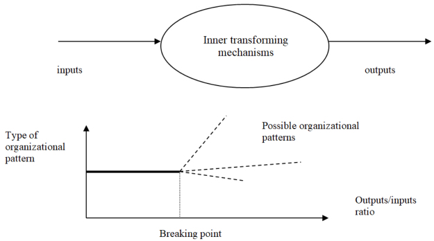
Figure 3.12. Bifurcation and change in organizational patterns
3.4.2.2. Change management: the academic approach
In section 2.7, we explained that the many aspects of what is called the organization theory defy easy classification. We then categorized different approaches into structural and functional theories on one side and cognitive and functional theories on the other side. This classification was proposed from an enterprise point of view.
Organizational structures are found in many environments other than the enterprise. Other criteria have been considered to classify them according to their functions or goals, nature of technology employed, ways to achieve compliance or the beneficiary of the organization. D. Katz and R. Kahn (1978) use functions performed or goals sought as the criteria to categorize organizations. According to them, production or economic organizations (manufacturing, logistics, distribution, retailing) exist to provide goods and services for society, whereas pattern maintenance organizations (education systems) prepare people to smoothly and effectively integrate other organizations. The adaptive organization (research and development) creates knowledge and tests theories, while the managerial or political organization (regulatory agencies) attempts to control resources use and authority.
In order to keep track of the baseline ideas of management thought in the profuse variety of literature produced about organizations, it helps to distinguish between organization behavior and organization theory when organizational change, adjustment or reconfiguration is considered.
Organization behavior primarily deals with individual and group levels. It covers motivation, perception and decision-making at the individual level and group functions, processes, performance, leadership and team building at the group level.
Organization theory deals with organization level such as organization change and growth, planning, development and strategy. Management of conflicts between groups and/or organizational units is dealt with at the intersection of organization behavior and organization theory.
From the point of view of change, the metaphor of organizations as open systems subject to external pressures facing them has become an accepted mindset for guiding management thought. Several corpora of thought that have direct or indirect connections with the reasons why organizations have to change have developed. Let us review the main ones.
Contingency “theorists” strive to prescribe organizational designs and managerial actions most appropriate for specific situations. It is clearly a perspective as an offshoot of systems theory applied to the study of organizations for organizational analysis.
“Contingency” theorists have tended to examine organizational designs and managerial actions most appropriate for specific situations. They view the environment as a source of change in open systems. Simultaneously, they highlight the interdependence of size, environment, technology and managerial structure, and their compelling congruence for business success. P. Lawrence and J. Lorsch (1967) who pioneered this approach argued:
“Underlying this new approach is the idea that the internal functioning of organizations must be consistent with the demands of the organization’s tasks, technology or external environment and the needs of its members if the organization is to be effective. Rather than searching for the panacea of the one best way to organize under all conditions, investigators have more and more tended to examine the functioning of organizations in relation to the needs of their particular members and the external pressures facing them. Basically this approach seems to be leading to the development of a ‘contingency’ theory of organization with the appropriate internal states and processes of the organization upon external requirements and member needs”.
Another group of theorists viewed environments as all-powerful in determining the fate of organizations. Drawing on the work of Charles Darwin, this group presented an “ecology” model that portrays successful organizations as the fittest in a competitive arena, where rules are imposed by the environment. H. Aldrich (1979), in an influential book, argued:
“The population ecology model differs from traditional explanations of organizational change […] it focuses on the nature and distribution of resources in organizations’ environments as the central force in change, rather than on internal leadership or participation in decisionmaking”.
Organizations as open systems, like living organisms, depend on their environment for critical resources, and a key managerial task is the appropriate provision of human-socio-cultural and political, technical, functional and informational resources.
All the arguments developed by different theorists converge to the point that organizational changes are induced or compelled by forces originating from organizations’ environments. The digital technology being introduced in all sectors of our societal context is a confirming and convincing example of this standpoint. It is a driving force for triggering deep reconfigurations of many an economic sector, beyond sheer adaptations. The interplay between the dynamical environment and current internal structures is a source of complexity to bring about a controlled evolution and to avoid disruptive situations running out of control.
3.4.2.3. Change management and social networks
3.4.2.3.1. General overview
If we hark back to section 2.3.2, an organization that is a purposive system is defined as a network representing a social structure directed toward some goal and created by communication between groups and/or individuals.
The nodes of a network can be embodied by BDI agents with their attributes in terms of beliefs, intentions and desires. This agent modeling can be used to guide change:
- 1) by conducting a comprehensive diagnosis before planning any course of action. Organizational change must not be targeted on a specific subsystem but must account for the total system dynamics, the system environment included. If a specific entity is created and assigned the responsibility of leading the change project, it has to be considered as an agent interacting with the other agents involved;
- 2) for prescribing phased action plans recognizing current patterns that feature the uniqueness of an organization and securing a departure from the search for one single optimal solution, all the more that patterns may change along with the project’s progress.
When relevant, the idea of “chunking” agents to be perceived as a single agent establishes a separate identity for the cluster within. According to context, one may wish to ignore the chunk’s internal structure or to take it into account. This allows a hierarchical approach to complex situations.
Affiliation networks (refer to section 2.3.1) are well-adapted tools to describe the properties of BDI agents’ networks in terms of beliefs, desires and intentions. Either the matrix formalism or n-partite graphs are eligible to represent real-world situations.
3.4.2.3.2. Long-range correlations
By analogy with the phenomena observed in physical systems, long-range effects can be observed in social networks. This is inductive to situations that can generate complex and chaotic configurations difficult to be understood by observers because they evolve fast and, as a result, should be dealt with by controllers, if any.
When analyzing a social network, a question arises: what is the size of individual nodes to take into account? Dunbar’s number can help define a space of interaction, or at least become aware of its potential range. The British anthropologist R.I.M. Dunbar (Dunbar 1992; Dunbar 2003) suggested that a cognitive limit exists to the number of people with whom one can maintain stable social relationships in which an individual knows who each person is and how each person relates to every other person. The average value for this number proposed by R.I.M. Dunbar is 148 for social group members. He also noted that group sizes could be put in three categories, namely 30–50 (bands), 100–200 (cultural lineage groups) and 500–2,500 (tribes).
It has become of interest in anthropology, evolutionary psychology, statistics and business management. Developers of social software are interested in it as they need to know the size of social networks that their software package is intended to support. In the modern military operational environment, psychologists seek such data to support or refute policies to maintain or improve unit cohesion. The application of Dunbar’s number to individual-centered and group-centered social networks has been validated (Gonçalves 2011).
When conducting a change management project, this dimension should be considered and integrated in the spectrum of parameters to deal with.
3.4.2.3.3. Some guidelines to conduct a change project with social agent networks
The basic idea governing the use of social networks to conduct a change project is to identify the change agents and to focus on their behavioral evolution. Agents as the project progresses can change behaviors: this has to be taken into account when monitoring a project.
When modeling social agents as BDI agents, their operational interactions should be represented by their action plans that reflect their activities within the framework of overall task distributions of the organization. An important category of change agents comprises the most connected. They can be identified when analyzing the traffic of incoming and outgoing messages. Each nodal agent sends messages to its contacts and receives messages from its contacts. For each nodal agent, the numbers of messages broadcast and received are captured over a period of time relevant to the context and display on a graph to visualize the results and help the understanding of the mesh of interrelations.
Nodal agents that send more messages than they receive are called “root” agents. They are of special interest because a change in their operations and plans will influence their roles more directly as broadcaster of changed messages. On the other hand, nodal agents receiving several messages must also get special attention because they have to be explained the new operational rules and must be assimilated so that their plans become aligned with what is intended by the change project.
This is a first-level analysis called the degree of connections in the agent network. It can be considered as a proxy for representing the flow of information inside the enterprise and with its outside partners. Never forget that organizations are open systems and their third-party partners (suppliers, clients) are full parts of the network. A second-level analysis is called the degree of closeness between the agents.
This second-level analysis refers to the beliefs and desires properties of BDI agents. They have to be polled to assess whether change is perceived as being a minor one or as having wide implications in terms of their own operations and their interaction with their closest partners. Specific courses of action have to be developed according to the situations of the different agents. All the features of BDI agents explained in the second part can be drawn on to carry such an analysis and deploy appropriate courses of action. This second-level analysis should help detect potential long-range effects liable to trigger complex and/or chaotic behavior conducive to losing control of the project.
A third-level analysis refers to the degree of trust between the agents and the acting agent in charge of the change project. This acting agent has itself beliefs, desires and intentions turned into action plans. They result from the content of the change project to be implemented in terms of purposes and objectives to be deployed in the field. It has to have a high degree of closeness with all the network agents involved in the change project and deliver advice in a context of trust.
These guidelines are only intended to provide a framework and a roadmap when carrying out a change project using BDI agents as a modeling tool.
3.4.2.4. Change management, data deluge and information systems
Functional subsystems influence each other, but the informational subsystem plays a special role because all organizational changes are reflected in MIS (management information system), which provides communication and coordination between all functional subsystems through the control of resources.
Figure 3.13 depicts the interplay between resources and primary processes in a manufacturing enterprise. Information is singled out at the same time as a resource, which mirrors the functioning of business models and secures collaboration and cooperation between resource management units.

Figure 3.13. Role of information in controlling business resources in a manufacturing enterprise
Hereafter, we focus on the features of an informational subsystem, which have to receive special attention within the framework of a change management project.
Transmission of information-laden data takes place through both formal and informal channels.
The formal channel refers to what is called the MIS. Collecting, gathering, processing and transmitting data according to set procedures embodied in software programs and mirroring management tools are the functional capabilities of information systems.
The way business agents or groups of agents make use of information systems can deviate significantly from the intentions of their designers. Many reasons explained their attitudes: misunderstanding of new procedures, refusal to change existing practice, tighter control of activities by eavesdropping, breakdown of informal channels of communication and so on.
Formal elements of information about structures and operations are attractive to company management because they are tangible. They can be easily defined and measured. However, they are only half the story. Many informal communication channels parallel or short-circuit the “official” patterns of communication flows. They are based on trust between the stakeholders involved. In case of reorganizations, many companies reassign decision rights, rework the organization chart or set up knowledge-sharing systems – yet they do not see the results they expect. That is because they have ignored the more informal, intangible building blocks. Norms, commitments, mind sets and networks are essential in getting things done. They represent (and influence) the ways people think, feel, communicate and behave. When these intangibles become desynchronized with one another or with the more tangible building blocks, the organization falters.
The informational subsystem must be identified as a subsystem in itself because advances in technology have made it the hub of coordination between all other business functional subsystems and business partners (suppliers, clients).
The critical issues at stake are delays in data transmission as already described to shun untimely decisions and their consequences, and accuracy of disseminated data (the destructive effect of fake or biased news does not need to be proved anymore). If these issues are not brought under full control, the whole system may run out of control because counterproductive decisions are taken untimely, as shown in the section “emergent behaviors” with unintended consequences (hunting and oscillating).
In the next sections, we focus on information systems and their architecture challenge in the era of data deluge.
3.4.2.4.1. What is an information system for?
Even if they are not aware of the fact, information system designers posit, explicitly or implicitly, that information systems are a modeled vision of the business universe. Regardless of the assumptions made about the chosen representation of the business universe, information system constructs are intended to reflect how the enterprise is organized and how it operates in terms of transactions and control rules. This implies that business information systems contain, in one way or another, a description of the enterprise’s organizational structures, functioning mechanisms and deliverables. Thus, the contents of business information systems should include the descriptive accounts of operations, control rules and deliverables (products/services).
This ideal situation was not found in the operational field for a wide variety of reasons:
- – business information systems usually resulted from the integration of software modules by different vendors. By the way, software integrators have become the flagship products of some vendors such as Net Weaver by SAP. It turns out that this complexity seriously hinders a reasonable understanding of the whole system by the lay business actors;
- – The MIS are often the back-offices of other processing systems such as transaction processing systems. A transaction is a business operation modifying the state of an enterprise or a part thereof. Capturing, storing, processing, disseminating and reporting transaction data are the objectives of transaction processing systems. The MIS procedures and their meaning are most often impenetrable to the users of transaction systems so that their management becomes short-sighted.
In fact, very few business actors lend weight in gaining knowledge of end-to-end business processes and their associated procedures carried out by the supporting information system. They are prone to finding themselves destitute of relevant understanding of the situation when they have to make local decisions that often turn out to have global impacts business-wise.
ERP-labeled software packages have brought forward the understanding of business processes for developing effective and efficient information systems. The best way to elicit the relationship of business processes and information systems is to devise information systems with an explicit architecture. Architecture defines the function capabilities of the parts of a system and the specifications of the relationships between these parts.
Linking ERP business processes and information systems through a layer architecture of IS modules allows us to:
- – remove barriers across organizational structures;
- – make procedural structures more explicit and flexible;
- – help decision-makers simulate the impact of their decisions.
The layer-based architecture of information systems has brought about significant improvement in making the links between business operations and information systems more explicit. It must be adapted to the presence of data flows coming from networks of servers. In the first section, the main features of the traditional layer architecture of information systems are described so that in the second section, the new architecture can be clearly contrasted with the traditional one.
3.4.2.4.2. Traditional layer architecture of information systems
Layer architecture is based on layers of functional operations and strongly contrasts with a hierarchical architecture developed on management levels (strategy, tactics and operations).
In a layered architecture, the underlying layers relate to the implementation, that is, to the different types of resources, while the top layers relate to the business. Figure 3.6 shows a schematic example of a layered architecture. A business system may well have more or fewer layers than the ones shown in Figure 3.14, and it can also have layers in several dimensions, so that one layer can itself be layered.

Figure 3.14. An example of layered business system architecture
The basic principle of any layered architecture is the delivery of services to a layer by underlying layers. When standardization is looked for, formats of services provided are defined, not the very mechanisms engineered to supply services under consideration.
The major benefit derived from layer modeling is the versatility it has for focusing on “relevant” views of a complex system and to trace back, when required, relations with detailed or aggregated descriptions.
- – The resource layer contains the different concrete resources needed for realizing the organization. Here, human resources with different kinds of skills – education, management, experience and so on – and different types of equipment such as information systems and transmission and switching equipment are found.
- – The infrastructure layer consists of functions generic to the type of business being modeled. Here, functions to support network and services management processes, accounting processes, personnel administration, office administration, and so on are found.
- – The common business process layer contains internal processes generic to the type of business modeled. These internal processes can be used by many different business processes within the company being modeled. Some of these processes can be described as cooperative services allowing for a structured workflow between the various activities of a single business process or different business processes.
- – Finally, the business system layer consists of the different business processes. These processes must be chosen to provide the top management with synthesized views of the enterprise. These views should be described in terms of performance indicators able to trigger leverage on relevant operations.
In systems with a layered architecture, it is important to define the interfaces between the various layers. Object-oriented technology provides an elegant method of doing this. This approach will be reproduced by substituting object for activity.
Every layer is a composite set consisting only of its constituent activities. The interface to a layer is made up of the interfaces to its public activities. By public, it is meant here to be accessible from outside. How a layer can be used by layers higher up in the structure is an important architectural decision. There are several such types of layer relations to choose from. Here, we present two of them:
- – the use of activities in the lower layer is encapsulated in the activities of the higher layer. The design of the higher layers uses the public interfaces of the basic activity layer as primitives; this is because the interface is encapsulated in the overlying layer’s activities and can only be seen in these activities’ implementation parts. The interface should not be used in the documentation, which describes the interaction between activities in the higher layers. A larger business system consists of thousands of activities that communicate with one another in an extremely intensive way; by concealing the communication with underlying activities inside the activities in their own layer, all documentation will be simplified.
Since they are designed to be extensively reused, basic command activities should be managed in a very different way compared to business activities: they should be carefully tested before being released; they should not be allowed to change until all business activities dependent on them have also been changed and so on;
- – activities in the lower layer need not only be encapsulated in activities of the higher layer but can be used in the design documentation of the higher layer; however, they cannot be changed by the designers of the higher layer. The common business process layer grows and matures during the development of several different business subsystems. It should contain the common activities of an entire business, and it should, therefore, become relatively stable after a number of releases. The layer should be managed in a way different from the business system layer, but similar to the infrastructure layer. An important difference, compared to the objects in the infrastructure layer, is that it is necessary to show the activities in the common business subsystems. When designing a business subsystem, you may show the common business processes you are using, but you are not allowed to make any changes in them whatsoever. You are only allowed to make changes in your own activities, that is, activities to realize your business subsystem. If a common business activity is to be changed, all business subsystems using that activity will need to be changed at the same time.
Every layer can be divided into subsystems. The subsystems in the highest layer, if any, cover large business areas and are supposed to reflect the core business processes as viewed by the top management. They can be dependent on each other. In this case, they are interrelated through an activity or a process of the underlying layer.
Business system areas and layering are complementary. You can apply both techniques to describe a complex organization. First, you use the business system area technique to find the different business system areas and their associated processes, and then you develop underlying support processes within the framework of a layered architecture. The layers below the highest will be used for all of the business system areas.
Figure 3.15 describes the concrete example of a layered information system architecture pertaining to a manufacturing company. This architectural pattern can be easily adapted to other types of organizations.

Figure 3.15. Layered information system architecture for a manufacturing company
The specific features of a layered architecture are best understood by contrasting it with hierarchical information system architecture for a manufacturing company as depicted in Figure 3.16.
3.4.2.4.3. Prospective overview of the future structures of information systems
It is common saying that we are in an era of rapid digital transformation. All sections of society, individuals as well as businesses and public administrations are embarked on a stream of change in the ways we interact and communicate. Virtual environments, namely server platforms, will be the hubs of faceless human social life in a global economic competition field.

Figure 3.16. Hierarchical architecture of application systems for a manufacturing company
Businesses are already embedded in agent networks of a sort, and in the past decades, they had to adjust to their evolving environments. Increasingly more relations with their suppliers and clients have become paperless and what is called dematerialized. The data sources they feed them will drastically increase in the forecast future altogether by their number and variety (CRM, Web portals, emails, social networks, collaboration systems, HR portals). In particular, IoT sensors monitoring real-time manufactured products will generate large volumes of remote data inflows and will bring unstructured data to businesses in order to be adequately processed. New policies of data governance will have to be promoted and deployed for reaping the benefits of the availability of “data lakes”.
The upper layer (customer care) and the lower layer (resources management) of the I S architecture depicted in Figure 3.15 are expected to be the most impacted. Their configuration will go through a drastic disruption to meet the processing requirements appropriate for interacting electronically with clients (customer care) and suppliers (resources management) via portals, e-shops, EDI systems, IoT sensors and so on. Each agent of these layers (sales, order handling, problem handling, purchasing, inventory, etc.) will receive or send managed transferred files from/to other agents, which are either other in-house agents or the front office, the enterprise’s trading partners, clients or suppliers.
IT systems are purpose-built for supporting efficient collaboration between all the in-shore and off-shore stakeholders of the business entity. Three types of systems can be identified:
System of records (SoR)
They are the traditional EDP (electronic data processing) systems that manage structured data related to business operations (financials, payroll, CRM – customer relationship management (inventory, order entry, HR – human resources), product life cycle management).
They have been designed on the basis of management concepts such as MRP, ERP and CRM (Briffaut 2015). They include data storage and access systems. They are the authoritative source of enterprise data.
System of engagement (SoE)
This system consists of the front offices of a business with its clients on one side and its suppliers on the other side. It is device-centric and associated with a variety of communication channels ranging from unstructured data from call centers, mobile devices, IoT sensors and so on to structured data.
System of insight (SoI)
This system is designed to convert unstructured and heterogeneous data sets received from various sources into structured data that can be fed into the system of records to support decision-making.
IBM (2015) has designed an SoI building block model for offering an enterprise architecture to deal with incoming data flows. It is represented in Figure 3.17.

Figure 3.17. System of insight building blocks to manage incoming data flows from clients by IBM
The consume and collect blocks refer to extracting data from the transactional system that will be used in the decision-making process and to collecting and aggregating it in view of further processing. The analyze and report blocks are intended to make sense of incoming data streams and prepare them for feeding the detect and decide blocks. The detect capability refers to discovering the existence of an event or a situation that requires one to make decisions. The capability of the decide block is to engineer the appropriate steps for delivering a decision.
The same model can be used to architecture the interaction of an e-enabled enterprise with its suppliers. In this case, data are generated by in-house transactions and are transformed in prepared data to be sent to suppliers. It is clear that some in-house data sources correspond specifically to external data sources.
The SoR, SoE and SoI systems are subject to constant adaptation in order to be kept in line with the enterprise evolution. In order to keep their adaptation under control, they are generally configured within a framework that is called an enterprise architecture (EA). A wide variety of definitions have been given to this concept. Gartner in the IT glossary of enterprise architecture (gartner.com, retrieved July 29, 2013) defines it in the following terms:
“EA is a discipline for proactively and holistically leading enterprise responses to disruptive forces by identifying and analyzing the execution of change toward desired business vision and outcomes. EA delivers value by presenting business and IT leaders with signatureready recommendations for adjusting policies and projects to achieve target business outcomes that capitalize on relevant business disruption. EA is used to steer decision-making toward the evolution of the future state architecture”.
Traditionally, the role of the IS system within the framework of a business approach is visualized as shown in Figure 3.18.
When a business unit is described as a system, the purpose is controlling its business operations. Three entities have to be identified: the controlled system, the controlling system and the information system. The controlled system, often called the transformation system, because it converts inputs into outputs, is generally modeled as a process. The relationships between these three entities are explicit from Figure 3.18. (for more details, see Briffaut (2015)).
It is noteworthy to elaborate Figure 3.18 to understand the features of the system approach to business description and especially the meaning of direct and indirect control. Direct control refers to direct action on the controlled process to maintain or change its state. Indirect control resorts to some entity external to the system to influence the state of the controlled process by means of inputs.
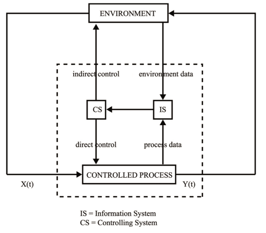
Figure 3.18. Articulation between controlled process, information system and controlling (decision) system in a manufacturing context with a cybernetic approach
Let us take an example in a manufacturing context to explain how the messages exchanged between the involved entities are connected and how their contents trigger decisions. The controlled process is assumed to be a manufacturing process made of storage and production activities. A message coming from the market place (environment data) is captured and processed by the information system (IS). The message content says that a market slump is forecast. It is directed to the production scheduler in an appropriate format (control data). As a result, the scheduler decides to reduce the production level by releasing orders to the manufacturing shops (direct control) on the basis of inventory levels (process data) and to send orders to suppliers to decrease the number of deliveries (indirect control).
What has to be changed to cope with an e-enabled context of digital interaction with clients and suppliers and of big data flows? The answer is straightforward: indirect control messages and environment data flows have to go through a layered system of SoE, SoI and SoR, as sketched in Figure 3.19.

Figure 3.19. Articulation between controlled process, information systems and controlling (decision) system in an e-enabled and data deluge context
3.4.2.4.4. Complexity of data governance and management
Data governance and management are key issues in a data deluge environment. The situation fits in what is described as a complex system. Three clusters of agents are in interaction, namely the end users of business data, the specialists in charge of delivering services to the end users and the technical infrastructure of data servers and telecommunication facilities. All these agents have to come to terms dynamically in an economic and technical context, which is always on the move. Each cluster has its operating rules, and synchronization of requirements between the clusters is not always, not to say often, effective. It is easy to figure out that this situation generates not only frictions between the stakeholders but also potential chaos, which can go out of control.
The business end users are considered owners of their data and as such demand to have simplified and facilitated access to their data 24/24 and 7/7 or according to SLAs (service-level agreements). When they detect that they require new data or new patterns of managed data, they put pressure on IT specialists to get what they want as soon as possible. This time to delivery can generate frustrations.
The number of data specialists involved in data processing and associated services is such that efficient collaboration between them is not straightforward: data preparation (appropriate data coding), database architecture, data analytics, real-time data provisioning to end users (data science). Scalability through modular systems has also become a key performance indicator to assess the quality of data management.
The infrastructure refers to computing and storage capacities on the one hand and to telecommunication facilities on the other hand.
The matching between these three agents clusters has to be secured through an adequate organizational structure all the more so when the technical infrastructure and data processing (application programs and databases) evolve under the pressure of end users’ requirements and the availability of new technologies. Managing the evolution of a legacy system is a daunting challenge. In many cases, it is not well-documented and changing the properties of a subsystem can generate chaos going out of control.
Systems learn more easily by removing parts. In general, we know what is wrong with more clarity than what is right, and our knowledge grows by subtraction. Actions that remove are more robust than those that add because addition may have unseen, complex feedback loops. Adding a new component to a system increases the number of interactions in the system, the nature of which may be uncertain and may not be maintained in terms of functions over time. This approach “learning by subtraction” is explicitly or implicitly used to deal with complex evolving systems.
3.4.2.4.5. Specific features of manufacturing information systems
Manufacturing corporations are faced with specific situations. A buzzword found in the technical press and bruited at conferences organized by a wide spectrum of stakeholders revolving about this industrial sector is digitalizing manufacturing. Examples of this broad notion are 3D printing, the Internet of Things (IoT), mass customization and last but not least big data or data deluge. In fact, this paradigm aims to marry information and communication technology to the process by which highly complex products are designed, manufactured and delivered to the final customer. Data flows add a massive amount of leverage in advanced manufacturing.
Information technology in advanced manufacturing
Large technology companies operate what can be called a digital factory where the real world, hardware and software merged with the virtual world, where simulation software elements allow us to assess whether the designed product meets the operational requirements set by the designers and can be manufactured with the equipment units and competencies available in the company.
The concept of CIM (computer-integrated manufacturing) was introduced by IBM in the seventies of the past century. The basic idea was to memorize in one database all the specifications of products in terms of materials contents and manufacturing operations associated with equipment units. Figure 3.20 describes the main features of this concept.
Let us explain the main functions and their relationships. The mission of the product development function is to design products in terms of components, materials required to manufacture final products either manufactured in-house or obtained from third-party suppliers (BM – Bill of Materials) and manufacturing operations expressed as programs for numerically controlled (NC) tools according to a routing appropriate to the job shop layout.
Customer orders are collected by the sales department, and their fulfillment is scheduled for making cost-efficient use of manufacturing resources. The implementation of schedules triggers the materials requirement planning function so that manufacturing and procurement orders are released to meet the delivery due dates of production schedules of finished products.

Figure 3.20. Building blocks of the computer-integrated manufacturing (CIM) concept by IBM
A software package called PLM (Product Lifecycle Manufacturing) allows us to simulate production processes and robotics ahead of time for optimizing engineering, procedures, quality, load time and uptime in order to make production more flexible and reliable in terms of delivery lead times. Before a manufacturing line is built and operated, simulation allows one to not only reduce and bring under control the time to put a new product to the market (time to market), but also to operate the manufacturing line with limited downtimes.
Sensors collect real-time data to software packages about the states of production lines. These data are used for predictive maintenance. In order to fulfill customer orders on time with the level of quality committed, it is critical to rely on fully operative equipment as scheduled by planning. Conventional approaches to equipment maintenance establishes a schedule for inspecting and maintaining all the components of the equipment units. This schedule is fixed and is based on the mean time before failure for each of the components. In a connected multi-factory environment, analytics of maintenance data can be shared with other sections of the enterprise manufacturing facilities that use the same type of tool. Taking one step further, the data from an individual tool can be sent to the equipment vendor. This piece of information can initiate discussions about improvements and feed into the supplier’s delivery schedule.
Further, the concept of proactive maintenance does not stop at the factory wall. The challenge is to make meaningful analytics out of these data for the benefit of customers. Many people do not yet understand why customers would pay for information making use of the products they have bought, easier, better, less costly or more valuable when IoT is taken into account for interacting with vendors.
Sensors embedded in products deliver data that make sense in terms of optimized operations, utilization rate, predictive maintenance and better support to the user. This set of data can become the holy grail of innovation with the proviso that data analytics is carefully carried out by manufacturers. In fact, weak signals can be hidden in the main stream of data flows, and each type of weak signal can be relevant to different business stakeholders.
Data analytics gives a company a lot of information it can use to optimize and shorten the value chain. This value chain consists of the suppliers of your suppliers (supply network), your company, your customers and their customers (distribution network). The purpose is to make your products faster, more cost-efficient, more flexible in small lot sizes while providing customers with enhanced support.
The manufacturing company can cut out different links of its value chain because they provide the least value in the company’s value chain. Hence, it needs to be understood. Where is the manufacturing company in the global value chain? How can it remain a key link by providing more value than anyone else in the chain?
Customers do not look any longer for products but for the services delivered by products. This is a paradigm shift. Many manufacturing companies claim that they sell solutions, applications and comprehensive systems versus products, namely value to customers instead of function capabilities. Car manufacturers are a telling example with the Internet of Things for cars. A connected car is a digitized vehicle with a built-in wireless network enabling advanced information and entertainment systems, real-time location and routing services, vehicle-to-vehicle and vehicle-to-infrastructure communication systems and remote diagnosis and update applications. It is easy to figure out that this approach to market, especially remote diagnosis and update applications, not only entails complex organizational methods and the deployment of appropriate information systems for car manufacturers, but also generates flows of data that have to be processed and analyzed.
A state of mind different from B2C and B2B offerings is emerging, namely “business to society” enterprise (B2S). The B2S concept means to contribute to civil society’s development in the world through providing people with reliable, safe services and making life in cities more bearable. This may reveal a start for changing relationships between industry and civil society.
Company employees are a special part of society and as such have to be made aware of their roles with respect to the social community they belong to. As company members, they deliver products/services to meet the requirements of their community fellows, add value to the company inputs, allowing them to receive salaries and to make other economic actors active by fulfilling their own needs. The final purpose of any company is durability through sustainable courses of action and societal responsibility.
Industry 4.0
What is meant by Industry 4.0? Industry 4.0, as Industry 3.0 draws on telecommunication services based on the Internet protocol of communication between message emitters and receivers. Industry 3.0 refers to the automation of machines and processes monitored by a single computer platform associated with network facilities. Industry 4.0 covers the concept of systems run on interconnected platforms combining engineering and manufacturing that can deal with global networked organizations.
For the sake of clarity, access to a computer server to retrieve data-laden messages on requests with the Internet protocol was called Internet 1.0. When an additional service became available, namely the capability from a remote terminal to feed data into a computer server, this service was called Internet 2.0.
The manufacturing flow is organized to make small lot sizes to meet customer orders on demand. The software steers the manufacturing process so that small lot sizes can be delivered cost-efficiently, at the due date and with the quality level committed to the customer.
The manufacturing process is monitored by machines talking to machines. Production is stopped when a defect is detected so that finished products do not have to be re-worked in case failures are detected at the final stage: “do it right the first time” is the paradigm underlying the manufacturing procedures and layout.
Industry 4.0 is intended to take the cost of scale to zero: regardless of the lot size, the unit cost price is about the same. This technical situation offers the possibility to convert standardized products into customized products, allowing for a competitive advantage. A product whose specifications are sent via the Internet will be built to order. Specific labor skills are required. Cost-efficient 3D printing makes possible lot size of one, the dream of the just-in-time endeavor launched by the Japanese industry in the 1970s.
3.5. References
Aldrich, H. (1979). Organizations and Environments, Prentice Hall.
Box, G. and Jenkins, G. (1970). Time Series Analysis, Forecasting and Control, Holden Day, San Francisco.
Briffaut, J.P. (2015). E-enabled Operations Management, ISTE Ltd, London and John Wiley & Sons, New York.
Dunbar, R.I.M. (1992). Neocortex size as a constraint on group size in primates, Journal Human Evolution, vol. 22, pp. 469–493.
Dunbar, R.I.M. (2003). The Social Brain: Mind, Language and Society in Evolutionary Perspective, Annual Review Anthropology, vol. 32, pp. 163–181.
Feigenbaum, M. (1992). “Foreword” in Peitgen, H.O., Jürgens, H.–D., Chaos and Fractals, Saupe, Springer Verlag.
Gonçalves, B., Perra, N. and Verpignani, A. (2011). “Modeling Users’ Activity on Twitter Networks – Validation of Dunbar’s Number”, PLoS ONE, e22656, available at: www.plosone.org.
Granger, C.W.J. and Newbold, P. (1987). Forecasting Economic Time Series, Academic Press, New York.
IBM (2015). Systems of Insight for Digital Transformation, Red Books, SG24-8293-00.
Kahneman, D. (2012). Thinking, Fast and Slow, Penguin Books Ltd.
Katz, D. and Kahn, R. (1978). The Social Psychology of Organizations, John Wiley & Sons, New York.
Lawrence, P. and Lorsch, J. (1967). Organization and Environment, Division of Research Graduate School of Business Administration, Harvard University Press.
Ross Ashby, W. (1956). An Introduction to Cybernetics, Methuen, London and New York.
Rovelli, C. (2017). Reality is Not What it Seems: the Journey to Quantum Gravity, Penguin Books Ltd.
Taleb, N.N. (2005). Fooled by Randomness: the Hidden Role of Chance in Life and in the Markets, Random House Inc, New York.
Taleb, N.N. (2008). The Black Swan, Penguin Book Ltd.
Turing, A.M. (1952). “The Chemical Basis of Morphogenesis”, Philosphical Transactions of the Royal Society, London B, pp. 37–72.