When time-ordered series of measurements are analyzed to help forecast the future behaviors of all sorts of ecosystems, it is important to detect whether there is some underlying equation for the phenomenon observed or it is a stochastic phenomenon.

What is called the phase space of a system is the set of all instantaneous states available to a system. The attractor of a dynamical system is the subset of phase space towards which the system evolves as time elapses. It can be just a point or a limited set of points.

When an attractor exists, the trajectories of the time-ordered data points with connecting line segments are treated as fractals in the associated phase space. Fractals are geometric forms with irregular patterns that repeat themselves at different scales. The forms consist of fragments of varying size and orientation but similar shape. The fractal dimension of an attractor is a parameter which characterizes a part of its properties.

Dimension is the way to measure the effect of enlargement (scaling) on length, area, volume and fractal object. Scaling by a factor n of length is length multiplied by n, of area is area multiplied by n², of volume is volume multiplied by n³ and of d-dimensional object is object multiplied by n^d.

While dimension provides information about the scaling properties of an object, it does not deliver information about the very structure of the object. However, its value gives useful information about the presence of determinism in the phenomenon observed.

Many definitions of dimension have been produced since 1919 when F. Haussdorf proposed a definition that is a purely description of the geometry of the fractal set and does not lend itself to quantitative estimation (Haussdorf 1919). An intuitive definition is as an exponent relating the bulk (volume, mass, information, etc.) of an object to its size (linear distance).

Bulk ≈ Size^dimension or dimension ≈ [log (Bulk) / log (Size) ]_{size → 0}

Size → 0 implies that dimension is a local quantity.

Let X(t) be the time series derived from experimental measurements captured at regular intervals τ. Variables of the series are [X_k (k τ )] with k = 0,1….n-1 and take part in the dynamics of the phenomenon. Our intention is to reconstruct the dynamics of the phenomenon only on the basis of the knowledge of the series [X_k (k τ)].

If the plot of X_k+1 versus X_k does not show any structure (cloud of points) for increasing values of k, it can be reasonably deduced that the phenomenon is stochastic.

[X_k (k τ)] are defined in the phase space spanned by all the variables of the series, as time elapses. X_k (k τ) follows either a curve or fragments of curves called phase space trajectories. Useful conclusions about the geometric structure of these trajectories can be deduced by using a procedure suggested by Ruelle (1985).

In order to try to characterize the presence of underlying variables embedded in the finite sample of measured variables, we now consider the following sequence of k variables Xi of (k+1) dimensions defined at equidistant points with a time lag T, a multiple of τ.

X₀: [X(0), X(T), X(2T), ……………..X (kT)]

X₁: [X(τ), X(τ+T), X(τ+2T), …….….X(τ+kT)]

X₂: [X(2τ), X(2τ+T), X(2 τ+2T), ….. X(2 τ+kT)]

Xk-1 : [X((k-1)τ), X((k-1)τ+T), X((k-1)τ+2T),…… X((k-1)τ+(k-1)T)]

If T is properly chosen, the variables X_i can be reasonably supposed to be linearly independent and offer us the possibility of unfolding the system’s dynamics into a multidimensional phase space Xi .

When a reference point Xi is chosen and the distances │ Xi - Xj │ from all the remaining points are computed, the data points within a defined distance r from X_i are counted. Repeating the process for all values of i, the quantity C(r,k) can be obtained

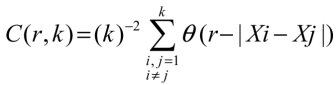
where θ(x) is the Heaviside function, θ(x) = 1 if x > 0 and θ(x) = 0 if x < 0.

C(r,k) is an integral correlation function of the attractor. It is expected to be proportional to r^d with d being the dimension of the attractor. d can be deduced from the plot of log C(r) versus log r.

What is explained above suggests the following procedure:

• – starting from the time series of measurements, deriving the integral correlation function C(r,k) of pairwise distances by considering successive higher values of the dimensionality k of phase space and different values of r whose minimum is the inter-point distance is computed;
• – when the d versus k dependence is stabilized beyond a certain k, the system represented by the time series of measurements should possess an attractor whose dimensionality is the saturation value of d. The value of k beyond which stabilization appears represents the minimum number of variables required to model the attractor’s mechanism.

These conclusions complement the contents of section 7.4.1.4 where questions were expressed.

References

Eckman, J.P. and Ruelle, D. (1985). “Ergodic theory of chaos and strange attractors”, Reviews of Modern Physics, vol. 57, no. 3, p. 617.
Haussdorf, F. (1919). “Dimension und äuβeres Maβ”, Mathematische Annalen, vol. 79, nos 1–2, pp. 157–179.
Packard, N.H., Crutchfield, J.P., Farmer, J.D. and Shaw, R.S. (1980). “Geometry from a time series”, Physical Review Letters, vol. 45, pp. 712–716.