
5
Binary to M-ary Coding and M-ary to Signal Coding: On-line Codes
5.1. Presentation and typology
A digital message, as a sequence of binary or M-ary elements called “information symbols”, is an abstract representation. To transmit this message, a physical quantity is associated with it in the form of an electrical signal (or optical signal for transmissions over optical fiber). This chapter describes the on-line codes used for baseband transmissions, as well as their most important properties.
The binary to M-ary transcoding and the M-ary to signal coding consists (see Figure 5.1) in:
- – a proper rule which allows one to associate with the binary sequence {bn}, bn ∈ [0,1] a sequence {an} where the symbols an belong to an alphabet of cardinal M > 2. This is called transcoding. Its essential purpose is to promote the operation that will follow (on-line code). This rule can be described in several ways: by a dictionary of codewords, by graph or state diagram;
- – an on-line coding which consists in constructing from each element an a waveform signal which occupies a time slice of at most T (with some exceptions) and which supports the symbol a. The signal thus formed at the output of the encoder is a so-called “baseband” signal. It is written:
where x(t) is a deterministic signal of a given pattern on the temporal interval [0, T[. A very common pattern for x(t) is that of a rectangular signal (pulse) of V amplitude:

Figure 5.1. Principle of binary to M-ary transcoding and M-ary to signal coding
The bitrate D (bit/s) of sequence bn is defined by the number of bits sent per unit of time. In synchronous digital transmission (our object), the transmission of bits by the source is done at a rate of one bit every Tb seconds:
Usually, binary to M-ary coding consists in associating with each word of k binary elements, a symbol an, with:
symmetric M-ary symbols. Knowing that:
the symbol rate Ds is then related to the bitrate by:
This allows that, at a given bitrate D, the symbol rate is reduced by increasing the number of levels M.
On-line codes can be classified according to the following typology:
- – linear codes: NRZ-L, NRZ-M, RZ, polar RZ, biphase (Manchester), biphase-M (differential), and partial response linear codes;
- – non-linear codes: non-alphabetic codes (Miller, bipolar RZ (AMI), CMI, HDB-n) and alphabetic codes.
Alphabetic codes will not be described in this book.
5.2. Criteria for choosing an on-line code
For baseband transmissions, the transmission medium consists of a cable (two-wire, coaxial, optical fiber) characterized by a limited bandwidth B of the “low-pass” type. It is necessary to use on-line codes whose characteristics are compatible with the properties of the transmission medium. The choice of a code therefore depends on the good properties that the code must have and which are essentially:
- – not to have a continuous component. Thus it will not be necessary to regenerate the continuous component and it will therefore be possible to add a supply voltage to the signal se (t) which will make it possible to remotely supply the repeater-regenerators (equipment located at each end of a section of an electric transmission cable);
- – to only have a little power at low frequencies because of the significant non-linear distortions and problems related to the separation of the continuous component of remote power supply of the repeater-regenerators with the spectral components of the on-line signal;
- – to prevent the spectrum of the transmitted signal from being much wider than the bandwidth B of the transmission channel, despite the pre-equalization which is carried out just before transmission. This also reduces crosstalk;
- – to allow the easy recovery of the transmission rhythm (clock recovery) for the synchronization of the receiver on the received signal;
- – to allow a transparent transmission: all sequences of binary information are authorized on transmission (for example, for a bipolar code the source cannot emit long sequences of “0” because it would generate at the reception a loss of the rhythm, hence the use of the code HDB-n: high-density bipolar of order n);
- – to have a certain redundancy allowing, among other things, one to monitor the quality of the transmission line without knowing the information sequence transmitted (for example, the use of 4B-3T coding).
The criteria for choosing an on-line code depend in part on its spectral properties. It is therefore necessary to know the power spectral density of an on-line code.
5.3. Power spectral densities (PSD) of on-line codes
The power spectral density ΓSe (f) of the signal se (t) is calculated in a precise way by the Fourier transform of its autocorrelation function RSe (t) (generally, this latter is rather difficult to calculate):

NOTE.– In problems 17 and 18 of the second volume of this book we have detailed, in the general case, the calculation of the autocorrelation function by probabilistic approach and the associated power spectral density of the RZ, NRZ and bipolar RZ on-line codes.
Furthermore, we show that the random data signals used in practice are cyclo-stationary signals (also called periodically “stationary”) of period T, so each statistical moment is replaced by its time average calculated over a period T. This will allow us to calculate their power spectral density.
The signal se(t) of the relation [5.1] at the output of the encoder can be interpreted as the result of the filtering of a signal a(t) by a filter whose impulse response is x(t):
with:
The sign ⨁ is the convolution operator.
The power spectral density ΓSe (f) of the signal se (t) is then: ΓSe(f) = ra(f)x X(f)2
Where Γa(f) is the power spectral density of the signal a(t), which will be calculated by the Fourier transform of its autocorrelation function, and X (/) is the Fourier transform of x(t). Γa(f) makes it possible to have a second degree of freedom (the first degree of freedom being the waveform x(t)) to control and shape the power spectral density of the on-line code.
In the case of partial response codes, which are part of the linear codes, we show that the calculation of the power spectral density ΓSe (f) of the signal se (t) is easily performed from an analogous expression to that given by relation [5.10], as the construction of these codes is carried out from four successive procedures.
Also, we must remember that a code is linear if the coding rule is a digital filtering operation (FIR or IIR filter) or a simple affine transformation.
For example:
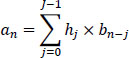
The set of coefficients hj that are integers, j ϵ [0,1,...,J — 1], defines the code.
5.4. Description and spectral characterization of the main linear on-line codes with successive independent symbols
These are codes such as:
They are more like a technique for shaping pulses than real coding. We also assume for these codes that the binary elements emitted at times nTb are independent and identically distributed (iid) on the alphabet {0,1} with:
The successive symbols an are independent because bn are.
Hereinafter, we describe the main independent successive symbol on-line codes and their spectral characteristics.
NOTE.– On all the chronograms of the various on-line codes that we describe, the bits are taken into account in the middle of the time interval by the clock (Ck) (as in reception) and the power spectral densities are represented for an average power of the on-line code equal to 1 (Pm = 1).
5.4.1. Binary NRZ code (non-return to zero): two-level code, two types of code
5.4.1.1. NRZ-L code "level code"
The NRZ-L code is defined by:
and:
With an = -1, the emitted signal is symmetrical; if an = 0, the emitted signal is non-symmetrical.
The diagram of the encoder and decoder of the symmetrical NRZ-L code is given in Figure 5.2.
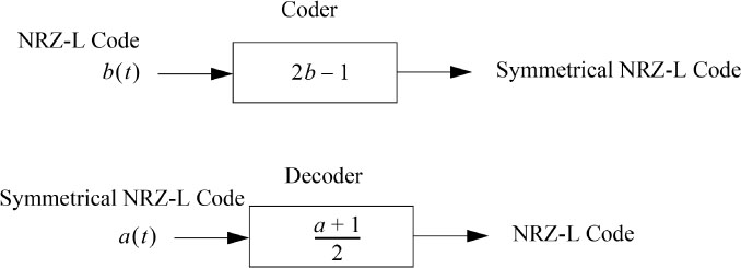
Figure 5.2. Diagram of encoder and decoder of the symmetrical NRZ-L code
In Figure 5.3, we present an example of a chronogram of the symmetrical NRZ-L code.
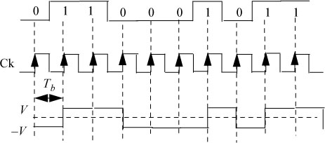
Figure 5.3. Example of a chronogram of the symmetrical NRZ-L code
Since the symbols an are iid (independent and identical distributed), its mean is zero and its variance σ2a is equal to 1.
The power spectral density of code NRZ-L is given by the following relationships:
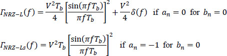
Figure 5.4 displays the power spectral density of the symmetrical NRZ-L on-line code. It consists of a main lobe which occupies the frequency band [0, 1/Tb] (for positive frequencies), and by an infinity of secondary lobes whose amplitude tends towards zero as the frequency increases. In addition, the PSD of this code is canceled at frequencies f = (k/T) with k non-zero integer.
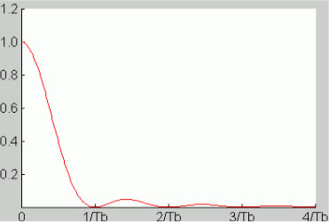
Figure 5.4. Power spectral density of the symmetrical NRZ-L on-line code. For a color version of this figure, see www.iste.co.uk/assad/digital1.zip
5.4.1.2. NRZ-M code “mark” or differential
The NRZ-M code is defined by the relation [5.17] and Table 5.1:
Table 5.1. Characterization of the NRZ-M code as a coding and decoding table
bn | an-1 | an |
| 0 | 0 | 0 |
| 0 | 1 | 1 |
| 1 | 0 | 1 |
| 1 | 1 | 0 |
The waveform x(t) and the power spectral density rNRZ-M(f) are identical to that of the symmetrical NRZ-L code.
In Figure 5.5, we give the block diagram of the on-line NRZ-M coder and decoder and an example of a chronogram of the symmetrical NRZ-M code is shown in Figure 5.6.
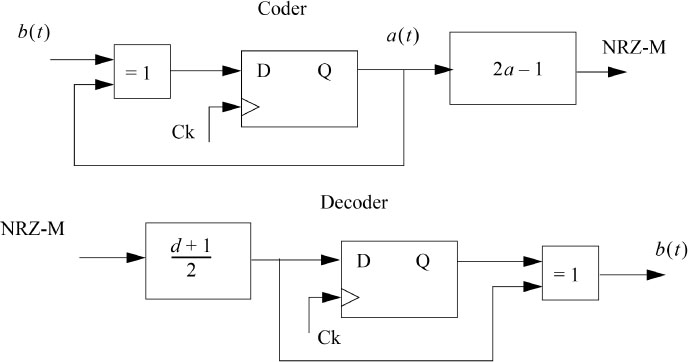
Figure 5.5. Block diagram of the NRZ-M coder and decoder
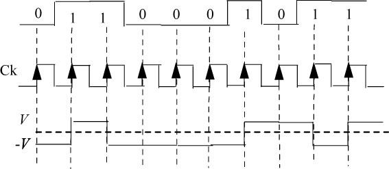
Figure 5.6. Example of a chronogram of the symmetrical NRZ-M code
5.4.2. NRZ M-ary code
The NRZ M-ary code is a generalization of the binary NRZ code. Each set of k bits from the binary sequence is associated with a symmetrical M-ary symbol:
The waveform x(t) is a “gate function” of amplitude V but of time duration T = kTb.
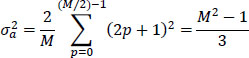
In the case where the symbols an are iid, then their mean is zero and their ![]() variance is equal to:
variance is equal to:
The power spectral density of the NRZ M-ary on-line code is:
Figure 5.7 shows an example of a chronogram of the NRZ 4-ary code with T = 2Tb, an = {± 1, ±3} and Figure 5.8 displays its power spectral density
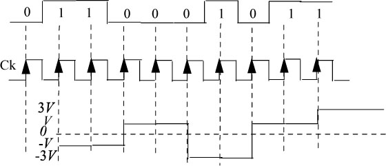
Figure 5.7. Example of the chronogram of the NRZ 4-ary on-line code
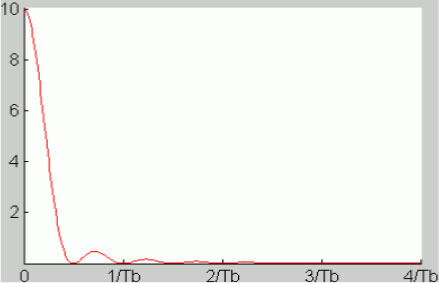
Figure 5.8. Power spectral density of the symmetrical NRZ 4-ary code. For a color version of this figure, see www.iste.co.uk/assad/digital1.zip
5.4.3. Binary RZ code (return to zero)
This refers to a two-level on-line code such as:
and:
with 0 < θ <1, in practice: θ — 1/2.
The binary RZ encoder corresponds to a multiplication operator between the binary sequence and the clock, as shown in Figure 5.9.
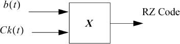
Figure 5.9. Diagram of the binary RZ on-line code (for θ — 1/2)
An example of a chronogram (for θ — 1/2) of this code is given in Figure 5.10.
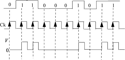
Figure 5.10. Example of a chronogram of the binary RZ code (for θ — 1/2)
The symbols an being independent and equiprobable, their mean is equal to 1/2 and their variance — 1/4. The power spectral density ΓRZ(f) is given by the following relation:

It consists of a continuous spectrum and of a discrete spectrum (discrete frequency components).
In general, one has θ = 1/2, hence:
As the relation [5.24] and Figure 5.11 show, the spectral occupancy of this on-line code is double that of the NRZ code and half of the power is located in the discrete components at frequencies (2k + 1)/Tb. We note in particular a discrete component at the frequency 1 /Tb, which does not have the NRZ code, which allows the recovery of the transmission rhythm (clock) at reception.
For θ = 1, the code is similar to the NRZ code but is asymmetrical, which results in the existence of a discrete component at f = 0 (so a non-null continuous component).
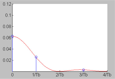
Figure 5.11. Power spectral density of the binary RZ on-line code (for θ = 1/2). For a color version of this figure, see www.iste.co.uk/assad/digital1.zip
5.4.4. Polar RZ on-line code
This refers to a 3-level on-line code:
and:
The block diagram of the encoder is given in Figure 5.12 for θ = 1/2.
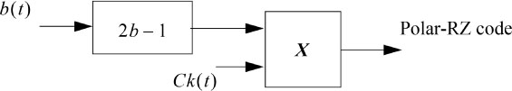
Figure 5.12. Block diagram of the encoder of the polar RZ on-line code (for θ = 1/2)
An example of a chronogram for this code is given in Figure 5.13 for θ = 1/2.
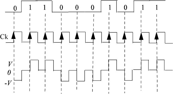
Figure 5.13. RZ polar code (for θ = 1/2)
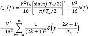
The power spectral density of this code is:
The spectrum has no discrete components and its continuous part is identical, except to a factor, to that of the RZ codes.
For θ = 1/2, the PSD is given by the relation [5.28]:
It is displayed in Figure 5.14.
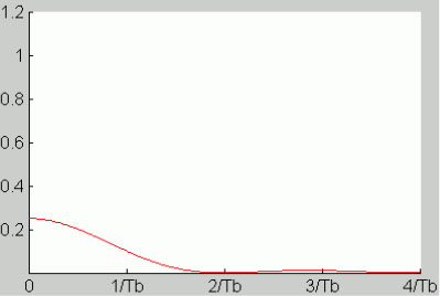
Figure 5.14. Power spectral density of the polar RZ code (for θ — 1/2). For a color version of this figure, see www.iste.co.uk/assad/digital1.zip
5.4.5. Binary biphase on-line code (Manchester code)
This is a two-level on-line code obtained by transmitting two opposite polarities during the time interval Tb corresponding to a binary symbol, each of these opposite polarities occupying a duration equal to Tb/2.
It is defined by:
and:
This code always has transitions (+V,-V or vice versa) in the middle of each interval of time duration Tb, regardless of the value transmitted (0 or 1). In addition, for the bit “0” there is a transition at the start of the interval. This is not the case for the bit “1”. The transitions are intended to limit the power in the vicinity of frequency zero. They make it possible to recover the clock at reception.
Figure 5.15 displays the block diagram of the binary biphase coder and decoder and Figure 5.16 shows an example of a chronogram of the biphase on-line code.
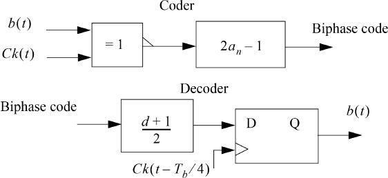
Figure 5.15. Binary biphase coder and decoder block diagram (Manchester code)
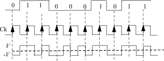
Figure 5.16. Example of a biphase code chronogram (Manchester code)
Since the symbols an are independent and equiprobable, of zero mean and of unit variance, the power spectral density of the code is:
This is displayed in Figure 5.17. It vanishes at zero frequency and remains relatively low for frequencies less than 1/4Tb. Therefore, this on-line code can be used for relatively long distance cable transmission.
However, the spectral occupancy of the code is double that of the NRZ code.
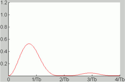
Figure 5.17. Power spectral density of a biphase code (Manchester code). For a color version of this figure, see www.iste.co.uk/assad/digital1.zip
5.4.6. Binary biphase mark or differential code (Manchester mark code)
The crossing of the transmission wires for a biphase code is equivalent for the receiver to an inversion of polarity and therefore to the inversion of the value of the binary symbols.
To avoid having to locate the line wires, it is preferred to use its differential variant: the differential biphase binary code. In addition, the latter offers better immunity against noise.
Note that all Ethernet systems use this type of on-line code, mainly in the MAC channel access control layer.
The differential biphase code uses the same symbols as the biphase code, but is coded differentially:
and:
The block diagram of the coder and the decoder is given in Figure 5.18 and an example of a chronogram of this code is given in Figure 5.19.

Figure 5.18. Block diagram of the differential biphase coder and decoder (Manchester mark code)
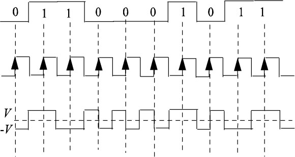
Figure 5.19. Example of a chronogram of the differential biphase code(Manchester mark code)
The power spectral density of the code is identical to that of the biphase code, so its spectral occupancy is therefore twice that of the NRZ code.
5.5. Description and spectral characterization of the main on-line non-linear and non-alphabetic codes with successive dependent symbols
These are on-line codes with dependent an symbols, although the message source remains with iid binary symbols.
5.5.1. Miller’s code
The spectral occupancy of this code derived from the biphase code is relatively reduced compared to the previous codes. Miller’s code is obtained by “dividing by two” the biphase coded signal. The state change of the Miller code is done on rising edges of the biphase code (from the example of the chronogram of Figure 5.21), but it can also be done on falling edges of the biphase signal.
Decoding consists of detecting the presence or absence of transitions in the middle of the symbol interval. The presence of transition corresponds to a state of the symbol. The absence of transition indicates the opposite symbol state.
The encoder block diagram is given in Figure 5.20 and an example of a chronogram for this code is given in Figure 5.21.
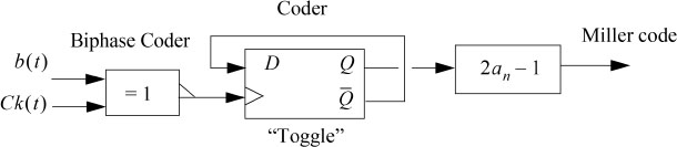
Figure 5.20. Block diagram of the Miller encoder
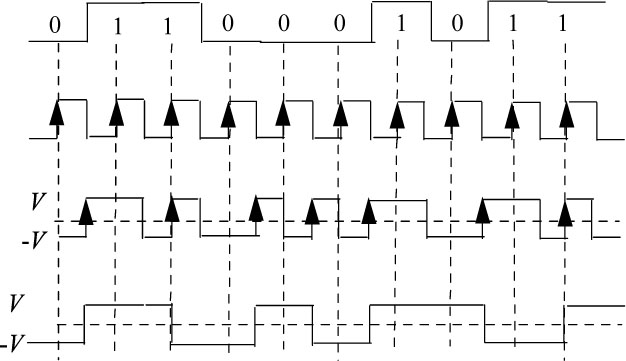
Figure 5.21. Example of a chronogram of the Miller code
The power spectral density of this on-line code is:
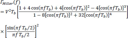
It is given in Figure 5.22. It is characterized by a high concentration of power in the vicinity of the frequency 2/5Tb. The power spectral density (which is here a continuous function) has a low value, but not zero at zero frequency, and the tolerance of the signal to the noise is reduced. However, Miller’s code allows the transmission of bitrates up to 5,000 bit/s over telephone cable.
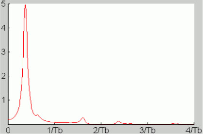
Figure 5.22. Power spectral density of the Miller on-line code. For a color version of this figure, see www.iste.co.uk/assad/digital1.zip
5.5.2. Bipolar RZ code or AMI code (alternate marked inversion)
This is a three-level on-line code such as:
The correlation of the symbols an is carried out by alternately assigning the values +1 and -1 to the symbols an when the binary symbol bn = 1.
The mean value of the symbols an is zero and their variance ![]() is equal to 1/2. The signal x(t) is defined by:
is equal to 1/2. The signal x(t) is defined by:
Or by:
to obtain the NRZ bipolar on-line code.
In Figure 5.23, we show the block diagram of the encoder and decoder of the bipolar RZ code and in Figure 5.24 we present an example of a chronogram of this code.
The power spectral density of the bipolar RZ code is:
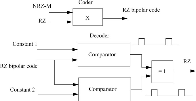
Figure 5.23. Block diagram of the bipolar RZ encoder and decoder (or AMI)
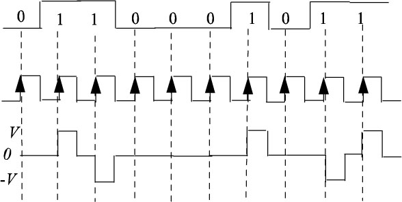
Figure 5.24. Example of a chronogram of the bipolar RZ code (or AMI)
Equation [5.38] is shown in Figure 5.25. We notice that the PSD is zero at zero frequency and does not have a discrete component at zero frequency (advantage for remote power supply). The spectral occupancy of the code is practically 1/Tb.
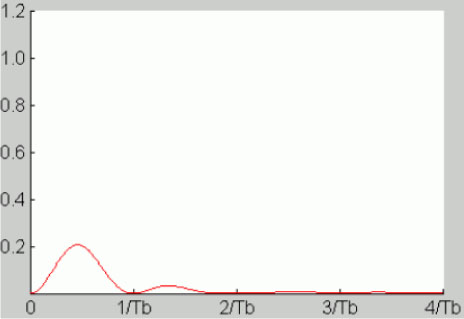
Figure 5.25. Power spectral density of the bipolar RZ code (or AMI). For a color version of this figure, see www.iste.co.uk/assad/digital1.zip
Furthermore, by performing a full-wave rectification of the bipolar RZ code, a binary RZ code is obtained which has a discrete component at frequency 1/Tb in its power spectral density and, consequently, an easy recovery of the clock at reception.
This code can be used on cables, but since the coding of the binary symbol “0” corresponds to a null signal emitted, this makes it difficult to recover the clock when sending long sequences of “0”, because in this case the amplitude of the frequency component at 1/Tb decreases quite strongly and the power of the signal collected after filtering may become insufficient to ensure the recovery of the clock. This has led to the development of on-line codes which have the advantages of the bipolar code, and in addition the advantage of allowing a correct recovery of the clock at reception, whatever the sequence of bits sent by the information source. HDB-n on-line codes are good examples of this type of on-line code (n-order high density bipolar code).
5.5.3. CMI code (code mark inversion)
This refers to a two-level code that has the same coding rule as the bipolar code but with different pulse forms:
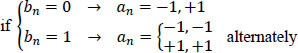
and:
An example of a CMI code chronogram is given in Figure 5.26.
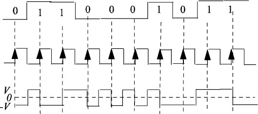
Figure 5.26. Example of a chronogram of a CMI code
The power spectral density of this on-line code is:
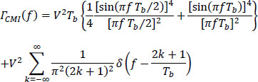
This is shown in Figure 5.27.
It is low at very low frequencies and has a discrete component at the frequency 1/Tb, so the clock recovery in reception is easy.
The only drawback is its higher spectral occupancy than that of the RZ bipolar code.
The CMI code has been proposed for the interface of 140 Mbit/s digital systems. It is also used in fiber optic transmissions.
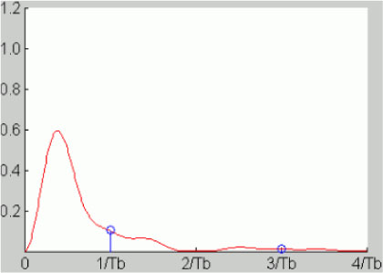
Figure 5.27. Power spectral density of the CMI on-line code. For a color version of this figure, see www.iste.co.uk/assad/digital1.zip
5.5.4. HDB-n code (high density bipolar on-line code of order n)
It is derived from the bipolar code in which any sequence of n + 1 consecutive zeros is replaced by a sequence of at most n consecutive zeros. For this, the (n + 1)th binary element of the n + 1 consecutive zeros sequence is coded by a symbol “7” (violation symbol) equal to ±1, the sign being chosen in such a way that it violates the rule of alternation. Also, in order to avoid the generation of a non-zero average, the violation symbols must themselves respect the rule of alternation between them.
However, it may be that the receiver cannot recognize a violation symbol as such (if it has a sign contrary to the previous 1); in this case, we code the first 0 of the sequence of n + 1 consecutive zeros with a symbol: an = ±1, of the same sign as the violation symbol which follows it. This symbol is called “stuffing symbol B".
IN SUMMARY.- A sequence “n + 1" zeros, 0 0..........0 0, is replaced by:
0 0..........0 V or by B 0.........0 V
with:
- – V: a symbol that violates the alternation rule of polarity, but satisfies the alternation rule of violation symbols between them;
- – B: a stuffing symbol that follows the alternation rule of polarity.
We give in Figure 5.28 an example of a chronogram of the code HDB-3.
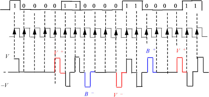
Figure 5.28. Example of a chronogram of the HDB-3 code. For a color version of this figure, see www.iste.co.uk/assad/digital1.zip
By doing so, the symbols always have a zero average. The analytical calculation of the power spectral density of the code HDB-n ΓHDB_n(f), is complicated. It is comparable to the power spectral density of the bipolar RZ code. Figure 5.29 shows the PSD of the HDB-3 code which is used in the DT1 and DT2 digital transmission systems.
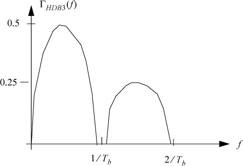
Figure 5.29. Power spectral density of the HDB-3 on-line code
In order to easily compare the spectral properties of the different on-line codes studied above, we have represented their power spectral density in Figure 5.30.
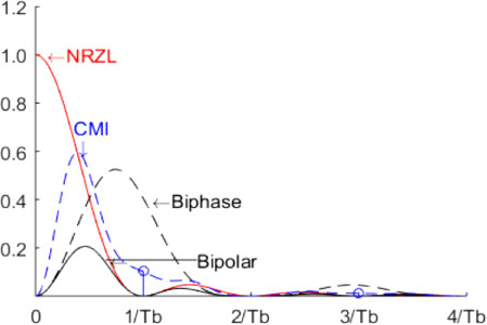
Figure 5.30. Power spectral density of the main on-line codes presented. For a color version of this figure, see www.iste.co.uk/assad/digital1.zip
5.6. Description and spectral characterization of partial response linear codes
These are multi-level linear codes that make it possible to easily modify and shape the spectrum of the signal to be transmitted in order to adapt it to the spectral characteristics of a baseband or equivalent low-pass transmission channel.
5.6.1. Generation and interest of precoding
Any partial response linear code can be generated from the sequence bn by means of four successive operations given in Figure 5.31.

Figure 5.31. Generation of partial response linear code
where:
NOTE.– For convenience and simplicity, we have limited the alphabet of an to two symbols. We could quite easily consider an alphabet with M = 2k symbols.
- – Precoding: the pre-coding operation makes the random sequence bn correspond to a random sequence b'n of the same bitrate and the same number of levels having certain advantages for decoding. Insofar as the symbols contained in bn are equiprobable and independent, the same goes for the sequence b'n.
- – Transcoding: the transcoding operation generates from the random sequence b'n a random sequence an of the same bitrate having a zero mean (symmetrical amplitude of the symbols with respect to zero).
- – Coding: the partial response linear encoding introduces a controlled inter-symbol dependency, which increases the number of signal levels and changes its spectrum. The encoding is similar to digital filtering. The encoder filter is characterized by its transfer function H(z).
- – Waveform shaping: waveform shaping is a filtering operation defined by an impulse response x(t) that determines the signal carrying the symbol of the transmitted signal se(t):
- – Interest of precoding: the advantage of precoding appears in the decoding procedure. Indeed, if the precoder has a transfer function P(z) which is the reverse of the transfer function H(z) modulo 2 of the coder, we will then have the block diagram of Figure 5.32.
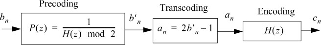
Figure 5.32. Precoder and encoder pair
Figure 5.32 shows that one goes from sequence bn to sequence b'n by the Z-transform filter: P(z). Then conversely, one goes from sequence b'n to sequence bn by the Z-transform filter: H(z).
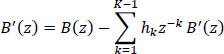
so one has:

and:
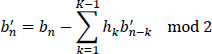
The coefficients hk are positive, negative or null integers, and h0 = 1. The FIR (finite impulse response filter) filtering of the encoder corresponds to algebraic operations. The preceding relationships show that on reception and in the absence of transmission noise, we can decode:
without needing to use the previous bn–k.
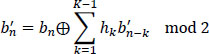
Otherwise, in the absence of precoding, (b'n — bn), we would have:
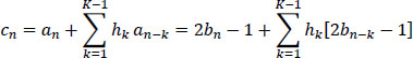
and decoding would be given by the relation:
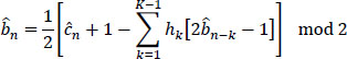
Therefore, the estimation of bn would require the estimation of the previous bn–k. In absolute terms, this would not be a problem, since they have already been estimated before bn. However, if they contain errors, then these will propagate.
5.6.2. Structure of the coder and precoder
5.6.2.1. Coder
The coder is defined by the following relation:
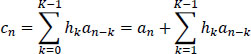
The Z-transform of cn is:
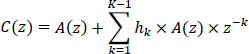
Hence, the transfer function of the filter is:
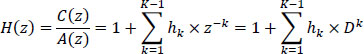
The coder filter is a FIR filter.
In the literature, the coder is often designated by a polynomial in D (delay operator, equivalent to the variable z–1 of the digital filtering).
The frequency response of the encoder filter is:
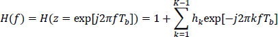
H(f) is a periodic function of period 1/Tb (Tb is the clock period).
The general structure of the encoder is given by relation [5.49] and presented in Figure 5.33.
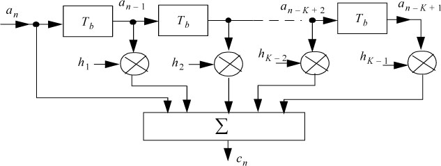
Figure 5.33. Block diagram of the general structure of the partial response linear encoder
5.6.2.2. Precoder
The precoder is a recursive filter whose transfer function is:
One can then write:
and:
or:
The structure of the precoder is generally given by relation [5.55], and presented in Figure 5.34. But as the alphabet of bn and b'n is {0,1}, then, in this case, the general structure of the precoder is also given by relation [5.56].
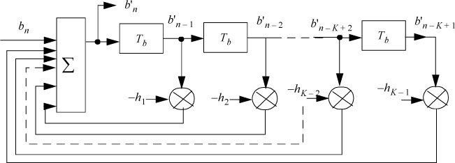
Figure 5.34. Block diagram of the general structure of the partial response precoder
5.6.2.3. Combined precoder and encoder
By comparing the block diagrams of Figures 5.33 and 5.34, it can be seen that the delay lines of the precoder and encoder can be shared according to the scheme of Figure 5.35.
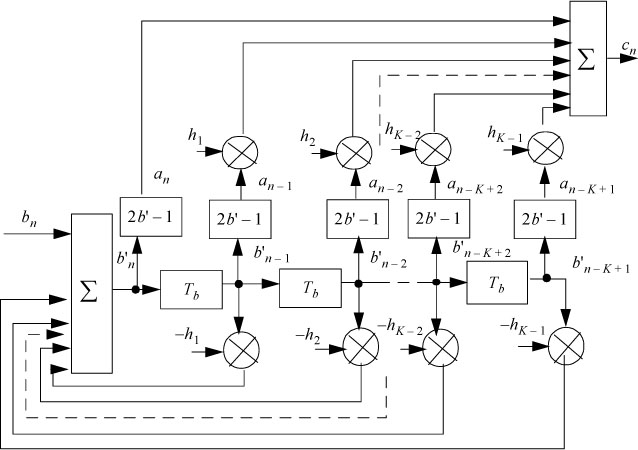
Figure 5.35. Combined structures of the precoder, transcoder and encoder
5.6.3. Power spectral density of partial response linear on-line code
To calculate the power spectral density of partial response linear on-line codes, we use the same approach described in section 5.3, by performing this block-by-block calculation according to the scheme of Figure 5.31, but by considering random signals instead of sequences, as shown in the block diagram of Figure 5.36.
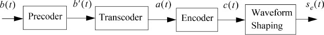
Figure 5.36. Block diagram of the generation of a partial response linear code for the calculation of the power spectral density
with:
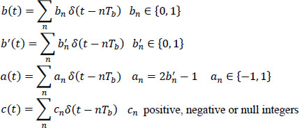
and δ(t) is the Dirac distribution (sometimes referred to as the “Dirac pulse”).
The random signals b(t), b'(t), a(t), c(t), se(t) are considered cyclo-stationary and have the power spectral densities: Γ'b(f), rb(f), ra(f), rc(f), rSe(f) respectively.
In this case, the autocorrelation function Rb(r) of the random sequence of distributions b'(t) (bn are assumed independent and equiprobable: iid) is given by:
And its power spectral density Γb(f) is given by:
The power spectral density Γb(f) of the random sequence of distributions b (t) is identical to that of b (t):
So, the precoding has no influence on the spectral properties of the code.
The autocorrelation function Ra (t) of the random sequence of distributions a(t) is given by:
In fact, the general relationship of Ra(t) with ane{—A,A} is:
The power spectral density Γa(f) of the random sequence of distributions a(t) is:
The power spectral density Γc(f) of the random sequence of distributions c(t) is:
And finally, the power spectral density of the signal emitted se(t) is given by:
This relation shows, on the one hand, that it is possible to shape the spectrum of the signal se(t) by modifying H(f) and, on the other hand, that the calculation of the spectrum is easy because it depends on the calculation of H(f) and X(f) separately.
5.6.4. Most common partial response linear on-line codes
The most common partial response linear on-line codes, such as duobinary, bipolar NRZ, interlaced bipolar of order 2 and biphase (WAL1 and WAL2), are described hereinafter following the approach used by Michel Stein (Stein 1991). The waveform shaping used is of the NRZ-L type.
5.6.4.1. Duobinary code
The duobinary code is characterized by:
K = 2 ; hi = 1
In which case, one has:
hence:
The encoder block diagram is given in Figure 5.37.

Figure 5.37. Duobinary encoder block diagram
The precoder is then defined by the following relation and the block diagram of Figure 5.38:
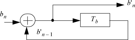
Figure 5.38. Duobinary precoder
The combined structure of the precoder, transcoder and duobinary encoder followed by the shaping function is shown in Figure 5.39.
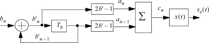
Figure 5.39. Combined structure of the precoder, transcoder and encoder of the duobinary on-line code
The graph of an example of a coded sequence is displayed in Figure 5.40.
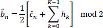
Note that ![]() mod 2 and the sample se(nT) of rank n makes it possible to determine ĉn and then bn (see Chapter 6).
mod 2 and the sample se(nT) of rank n makes it possible to determine ĉn and then bn (see Chapter 6).
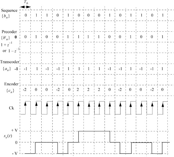
Figure 5.40. Example of duobinary on-line code
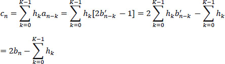
The spectral properties of the duobinary code are deduced from the transfer function of the encoder:
hence:
If ±V are the peak values of se (t), and the pulse x(t) has an amplitude V/2 on [0, Tb [, then:
and from [5.65], the power spectral density is:
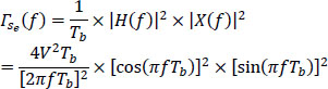
or:
It is displayed in Figure 5.41.
The power spectral density has a reduced bandwidth equal to 1/2Tb Hz (if we consider the positive frequencies only).
However, with the same peak amplitude, the change from two to three levels increases the sensitivity to noise.
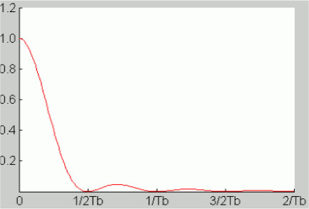
Figure 5.41. Power spectral density of duobinary on-line code. For a color version of this figure, see www.iste.co.uk/assad/digital1.zip
5.6.4.2. NRZ bipolar code
The bipolar code, the principle of which has been explained above, is seen here as a partial response linear code whose coding law is defined by:
K = 2 ; h1 = -1
In which case, one has:
hence:
The coder scheme is given in Figure 5.42.
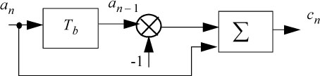
Figure 5.42. NRZ bipolar code block diagram
The precoder is identical to that of the duobinary code, and the set of precoder, transcoder, encoder and waveform shaping is shown in Figure 5.43.
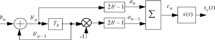
Figure 5.43. Combined block diagram of the precoder, transcoder, coder and waveform shaping of the nRz bipolar code
An example of a coded sequence is shown in Figure 5.44.
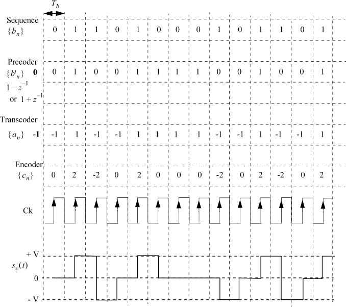
Figure 5.44. Example of a coded sequence of the NRZ bipolar on-line code
The transfer function of the encoder is:
And its power spectral density is calculated as follows:
hence:
Finally, one has:
This is displayed in Figure 5.45.
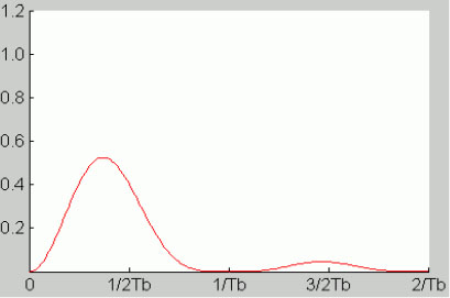
Figure 5.45. Power spectral density of the NRZ bipolar on-line code. For a color version of this figure, see www.iste.co.uk/assad/digital1.zip
5.6.4.3. Interleaved order 2 bipolar code
The interleaved bipolar coder of order 2 can be obtained by serializing duobinary and bipolar coders. The structure of the 2nd order interleaved bipolar coding chain is then represented in Figure 5.46, where H1(z) and H2(z) respectively represent the transfer functions of the duobinary and bipolar coders.
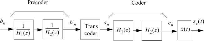
Figure 5.46. 2nd order interleaved bipolar coding structure
The transfer function and the impulse response of the encoder are written:
And the output of the encoder is expressed by:
The encoder block diagram is given in Figure 5.47. It is similar to that of the bipolar coder of Figure 5.42 by replacing the delay Tb by 2Tb.
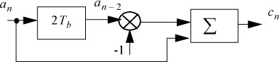
Figure 5.47. 2nd order interleaved bipolar code
The precoder is defined by the following relation:
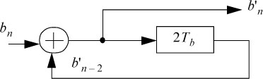
Figure 5.48. 2nd order interleaved bipolar precoder
Its implementation scheme is shown in Figure 5.48.
The whole chain of two-order interleaved bipolar coding is shown in Figure 5.49.
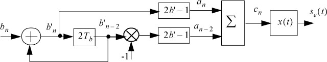
Figure 5.49. 2nd order interleaved bipolar coding chain
An example of a coded sequence is displayed in Figure 5.50.
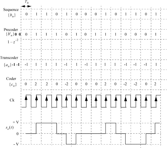
Figure 5.50. Example of a coded sequence of the 2nd order interleaved bipolar code
One can easily verify that the coding method illustrated in Figure 5.50 is equivalent to separately carrying out a bipolar coding on the sequence of the even bits {b2n} and on the sequence of odd bits {b2n+1} of the message to be transmitted {bn}. Then, the two coded sequences are interleaved so that the symbol corresponding to the bit of rank n occupies the same rank n in the coded signal.
The frequency response of the encoder is:
This is displayed in Figure 5.51.
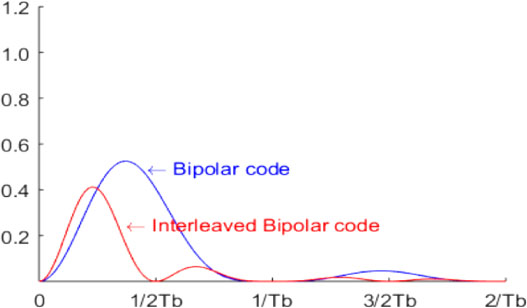
Figure 5.51. Power spectral density of the 2nd order interleaved bipolar codes and the simple bipolar code. For a color version of this figure, see www.iste.co.uk/assad/digital1.zip
5.6.4.4. Biphase codes
The spectral occupancy of the interleaved bipolar code of order 2 is half that of the simple bipolar code.
These codes are characterized by the inversion or not of a periodic carrier signal as a function of the binary element to be transmitted. The most used biphase code is that described previously and designated here by the term “WAL1”. Another variant, called “WAL2” can be used in which the carrier signal has a phase shifted by n/2 with respect to the series of bits. Figure 5.52 shows the two basic possible forms of signals in each variant.
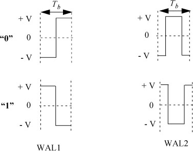
Figure 5.52. Basic signals used in biphase codes WAL1 and WAL2
The precoding operation for these codes is replaced by the identity transformation, therefore:
5.6.4.5. Biphase code WAL1
Its transfer function is given by:
and H(f) is given by:
then:
The shaping filter has a rectangular impulse response of width Tb/2. Its transfer function is therefore:
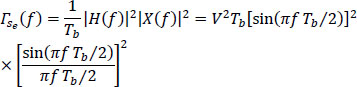
Hence, its power spectral density Γs (f) is given by:
The differential biphase code described above is obtained by putting a precoder defined by the following equation upstream of the coder:
5.6.4.6. Biphase code WAL2
The coding and shaping functions are:
and:
So one has:
The same precoder as for the WAL1 code allows differential coding.
The power spectral densities of the two-phase codes WAL1 and WAL2 are displayed in Figure 5.53.
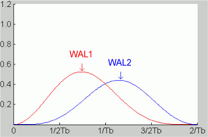
Figure 5.53. Power spectral densities of the two-phase codes WAL1 and WAL2. For a color version of this figure, see www.iste.co.uk/assad/digital1.zip
We note that the PSD of code WAL2 has very little energy at low frequencies and this part of the spectrum remains available for useful purposes (adding a voice channel, for example).
Finally, we have also displayed, in Figure 5.54, the power spectral density of the different partial response linear codes analyzed above, in order to allow an easy comparison of the power spectral density properties of these codes.

Figure 5.54. Power spectral density of on-line codes presented. For a color version of this figure, see www.iste.co.uk/assad/digital1.zip