One of the most common examples of broadcasting is the addition of a function and a constant; if C is a scalar, one often writes:

This is an abuse of notation since one should not be able to add functions and constants. Constants are however implicitly broadcast to functions. The broadcast version of the constant C is the function  defined by:

Now it makes sense to add two functions together:

We are not being pedantic for the sake of it, but because a similar situation may arise for arrays, as in the following code:

vector = arange(4) # array([0.,1.,2.,3.])
vector + 1.        # array([1.,2.,3.,4.])

In this example, everything happens as if the scalar 1. had been converted to an array of the same length as vector, that is, array([1.,1.,1.,1.]), and then added to vector.

This example is exceedingly simple, so we proceed to show less obvious situations.

A more intricate example of broadcasting arises when building functions of several variables. Suppose, for instance, that we were given two functions of one variable, f and g, and that we want to construct a new function F according to the formula:

This is clearly a valid mathematical definition. We would like to express this definition as the sum of two functions in two variables defined as

and now we may simply write:

The situation is similar to that arising when adding a column matrix and a row matrix:

C = arange(2).reshape(-1,1) # column
R = arange(2).reshape(1,-1) # row
C + R                       # valid addition: array([[0.,1.],[1.,2.]])

This is especially useful when sampling functions of two variables, as shown in section Typical examples.

We have seen how to add a function and a scalar and how to build a function of two variables from two functions of one variable. Let us now focus on the general mechanism that makes this possible. The general mechanism consists of two steps: reshaping and extending.

First, the function g is reshaped to a function  that takes two arguments. One of these arguments is a dummy argument, which we take to be zero, as a convention:

Mathematically, the domain of definition of is now Then the function f is reshaped in a way similar to:

Now both and take two arguments, although one of them is always zero. We proceed to the next step, extending. It is the same step that converted a constant into a constant function (refer to the constant function example).

The function  is extended to:

The function is extended to:

Now the function of two variables F, which was sloppily defined by F(x,y) = f(x) + g(y), may be defined without reference to its arguments:

For example, let us describe the preceding mechanism for constants. A constant is a scalar, that is, a function of zero arguments. The reshaping step is thus to define the function of one (empty) variable:

Now the extension step proceeds simply by:

The last ingredient is the convention on how to add the extra arguments to a function, that is, how the reshaping is automatically performed. By convention, a function is automatically reshaped by adding zeros on the left.

For example, if a function g of two arguments has to be reshaped to three arguments, the new function would be defined by:

When NumPy is given two arrays with different shapes, and is asked to perform an operation that would require the two shapes to be the same, both arrays are broadcast to a common shape.

Suppose the two arrays have shapes s₁ and s₂. This broadcasting is performed in two steps:

Suppose we want to add a vector of shape (3, ) to a matrix of shape (4, 3). The vector needs be broadcast. The first operation is a reshaping; the shape of the vector is converted from (3, ) to (1, 3). The second operation is an extension; the shape is converted from (1, 3) to (4, 3).

For instance, suppose a vector of size n is to be broadcast to the shape (m, n):

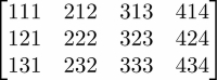
To demonstrate this we consider a matrix defined by:

M = array([[11, 12, 13, 14],
           [21, 22, 23, 24],
           [31, 32, 33, 34]])

and vector given by:

v = array([100, 200, 300, 400])

Now we may add M and v directly:

M + v # works directly

The result is this matrix:

It is not possible to automatically broadcast a vector v of length n to the shape (n,m). This is illustrated in the following figure:

The broadcasting will fail, because the shape (n,) may not be automatically broadcast to the shape (m, n). The solution is to manually reshape v to the shape (n,1). The broadcasting will now work as usual (by extension only):

M + v.reshape(-1,1)

Here is another example, define a matrix  by:

M = array([[11, 12, 13, 14],
           [21, 22, 23, 24],
           [31, 32, 33, 34]])

and a vector by:

v = array([100, 200, 300])

Now automatic broadcasting will fail, because automatic reshaping does not work:

M + v # shape mismatch error

The solution is thus to take care of the reshaping manually. What we want in that case is to add 1 on the right, that is, transform the vector into a column matrix. The broadcasting then works directly:

M + v.reshape(-1,1)

For the shape parameter -1, refer to section Accessing and changing the shape of Chapter 4, Linear Algebra  - Arrays. The result is this matrix:

Suppose M is an n × m matrix, and we want to multiply each row by a coefficient. The coefficients are stored in a vector coeff with n components. In that case, automatic reshaping will not work, and we have to execute:

rescaled = M*coeff.reshape(-1,1)

The setup is the same here, but we would like to rescale each column with a coefficient stored in a vector coeff of length m. In this case, automatic reshaping will work:

rescaled = M*coeff

Obviously, we may also do the reshaping manually and achieve the same result with:

rescaled = M*coeff.reshape(1,-1)

Suppose u and v are vectors and we want to form the matrix W with elements w_ij = u_i + v_j. This would correspond to the function F(x, y) = x + y. The matrix W is merely defined by:

W=u.reshape(-1,1) + v

If the vectors u and v are [0, 1] and [0, 1, 2] respectively, the result is:

More generally, suppose that we want to sample the function w(x, y) := cos(x) + sin(2y). Supposing that the vectors x and y are defined, the matrix w of sampled values is obtained by:

w = cos(x).reshape(-1,1) + sin(2*y)

Note that this is very frequently used in combination with ogrid. The vectors obtained from ogrid are already conveniently shaped for broadcasting. This allows for the following elegant sampling of the function cos(x) + sin(2y):

x,y = ogrid[0:1:3j,0:1:3j] 
# x,y are vectors with the contents of linspace(0,1,3)
w = cos(x) + sin(2*y)

The syntax of ogrid needs some explanation. First, ogrid is no function. It is an instance of a class with a __getitem__ method (refer to section Attributes in Chapter 8, Classes). That is why it is used with brackets instead of parentheses.

The two commands are equivalent:

x,y = ogrid[0:1:3j, 0:1:3j]
x,y = ogrid.__getitem__((slice(0, 1, 3j),slice(0, 1, 3j)))

The stride parameter in the preceding example is a complex number. This is to indicate that it is the number of steps instead of the step size. The rules for the stride parameter might be confusing at first glance:

Another example for the output of ogrid is a tuple with two arrays, which can be used for broadcasting:

x,y = ogrid[0:1:3j, 0:1:3j]

gives:

array([[ 0. ],
       [ 0.5],
       [ 1. ]])
array([[ 0. ,  0.5,  1. ]])

which is equivalent to:

x,y = ogrid[0:1.5:.5, 0:1.5:.5]