
This chapter will cover element and homogeneous data type vectors in more detail. The chapter will move from contiguous memory allocation to a non-contiguous memory allocation data type such as a linked list. The linked list data structure collects data and orders them relative to the other elements that come before and after it. The linear data structure can be thought of as having two ends, and the way an item is added or removed from the linear structure distinguishes one structure from another. The chapter will cover multiple variants of linked lists, such as linear linked lists, doubly linked lists, and circular linked lists. The chapter will introduce below mentioned topics in detail:
- Built-in data types in R, such as vector, and element data types
- Writing object-based programs using R S3, S4, and references classes
- Array-based list implementation
- Linked lists
- Comparison of list implementations
- Element implementations
- Doubly linked lists
- Circular linked lists
- Vector and atomic vector
Before we get into data structure concepts, let's look into data types provided by the R programming language. A basic data structure with a homogenous data type is based on a contiguous sequence of cells to enable fast access to any particular dataset. All homogeneous types support a single data type.
For example, in Figure 3.1 we have a numeric, logical, and character data type, however, it is stored as character.

Figure 3.1: Example of vector stored as character
Similarly, a matrix with multiple data types, as shown in Figure 3.2, will be coerced and stored as character data type. The array is an extension of the matrix from 2-D to n-D.

Figure 3.2: A matrix with numeric and characters are stored as 2D matrix with characters data type
All elements of a homogeneous data structure must be the same type, so R attempts to combine the different data types to the most flexible type in a priority order as shown in Figure 3.3:

Figure 3.3: Priority order of data types during coercion
Based on Figure 3.3, you can see that the character data type gets most priority in homogeneous data type. Logical gets converted into integer, and integer gets converted into numeric if the data type is homogenous. All these are built-in data structures. The following table shows coercion of different data types:

Figure 3.4: The table shows different types of vector coercions
The vector representation stores elements in contiguous memory allocation, and the cells are accessed through indexing such as v[2] denotes second element of vector v. R has six basic atomic vectors.
The following table lists all six basic atomic vectors with their modes and storage modes:

Figure 3.5: The table shows different modes and storage modes of atomic vector types
Contiguous memory allocation and access through indexing makes any insertion or deletion quite expensive. For example, say a company wants to manage the current working employees' details such as name, gender, age, department, and so on. For simplicity, let's only consider that we want to use a vector representation for storing the employee name. Let's assume m employees are currently present in the company, and a new employee named Navi joins the company. As employee names are stored in a sorted order, they have to store it after Bob, as shown in the following figure:

Figure 3.6: An example of insertion in vector
To perform this operation, all employee names need to be shifted by one, leading m-k operations to be performed where k is the insertion position in the vector. Similarly, in a deletion operation, all elements needs to be shifted back as shown in figure below:
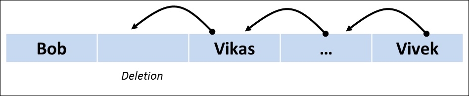
Figure 3.7: An example of deletion of element from vector
R supports various element data types, which have unique properties associated with them. Atomic vectors are the most elemental data types as covered under the preceding section. Other forms of data types are as follows:
A factor is a vector of integer values labeled to each corresponding set of unique characters in a categorical vector. The content within a factor can be of numeric or character format. The content can be of multiple forms such as character, numeric, logical, and complex.
The following example shows how the characters within a categorical vector have been uniquely auto-assigned to an integer (factors). The integer levels are assigned based on the sequence of occurrence of unique character elements within a vector.
> fact1 <- factor(c("a","b","c","c","a","b"))
> fact1
[1] a b c c a b
Levels: a b c
> str(fact1)
Factor w/ 3 levels "a","b","c": 1 2 3 3 1 2
However, it is possible for a user to define levels as per requirements:
> fact2 <-
factor(c("a","b","c","c","a","b"),labels=c(1,2,3),levels=c("c","a","b
"))
> fact2
[1] 2 3 1 1 2 3
Levels: 1 2 3
> str(fact2)
Factor w/ 3 levels "1","2","3": 2 3 1 1 2 3
A matrix is a two-dimensional array vector defined as rows and columns with homogenous content, which can be of multiple forms such as character, numeric, logical, and complex.
The following example shows a numeric and a character matrix. A mode() is used to check the data type as present in the R environment.
## Numeric Matrix
> mat1 <- matrix(1:10,nrow=5)
> mat1
   [,1] [,2]
[1,]    1    6
[2,]    2    7
[3,]    3    8
[4,]    4    9
[5,]    5   10
> mode(mat1)
[1] "numeric"
## Categorical Matrix
> mat2 <- matrix(c("ID","Total",1,10,2,45,3,26,4,8),ncol=2,byrow=T)
> mat2
  [,1] [,2]
[1,] "ID" "Total"
[2,] "1"  "10"
[3,] "2"  "45"
[4,] "3"  "26"
[5,] "4"  "8"
> mode(mat2)
[1] "character"
An array is an n dimensional vector with homogenous content, which can be of multiple forms such as character, numeric, logical, and complex.
The following example shows how to generate a three-dimensional array:
> arr1 <- array(1:18,c(3,2,3))
> arr1
, , 1
   [,1] [,2]
[1,]    1    4
[2,]    2    5
[3,]    3    6
, , 2
   [,1] [,2]
[1,]    7   10
[2,]    8   11
[3,]    9   12
, , 3
  [,1] [,2]
[1,]   13   16
[2,]   14   17
[3,]   15   18
The c(3, 2, 3) column vector defines the dimension of array in such a way that length of the column vector defines the dimension of the array and the values of the column vector define grid size. In this case, X has 3 units, Y has 2 units and Z dimension has 3 units.
A dataframe is a two-dimensional table with combinations of multiple forms of vectors (heterogeneous content) of equal length. It possesses properties of both list and matrix. The content can be of multiple forms such as character, numeric, logical, and complex.
The following is a dataframe with five observations and four attributes:
> Int <- c(1:5); Char <- letters[1:5];
Log <- c(T,F,F,T,F); Comp <- c(1i,1+2i,5,8i,4)
> data.frame(Int,Char,Log,Comp)
Int Char   Log Comp
1   1    a  TRUE 0+1i
2   2    b FALSE 1+2i
3   3    c FALSE 5+0i
4   4    d  TRUE 0+8i
5   5    e FALSE 4+0i
A list is a way of grouping all possible objects (including lists themselves) and assigning them to a single object. It has a one-dimensional property, which can take in heterogeneous objects. It is also called recursive, as it can contain multiple lists within one. The content can be of multiple forms such as character, numeric, logical, and complex.
The following code explains how to create a list, and what it it looks like in the R environment:
> list1 <- list(age = c(1:5), #numeric vector
+ name = c("John","Neil","Lisa","Jane"), #character vector
+ mat = matrix(1:9,nrow = 3), #numeric matrix
+ df = data.frame(name = c("John","Neil","Lisa","Jane"), gender =    c("M","M","F","F")), #data frame
+ small_list = list(city = c("Texas","New Delhi","London"), country    = c("USA","INDIA","UK"))) #list
> list1
$age
[1] 1 2 3 4 5
$name
[1] "John" "Neil" "Lisa" "Jane"
$mat
  [,1] [,2] [,3]
[1,]    1    4    7
[2,]    2    5    8
[3,]    3    6    9
$df
name gender
1 John      M
2 Neil      M
3 Lisa      F
4 Jane      F
$small_list
$small_list$city
[1] "Texas"  "New Delhi" "London"
$small_list$country
[1] "USA"   "INDIA" "UK"
R also supports multiple ways to implement data types using object-oriented programming (OOP) such as S3, S4, and R5 classes. The next section provides the basics on OOP, which will later be used for implementing different data structures.