
Memory efficiency is an important aspect to be considered while designing data structure and algorithms. Memory can be broadly classified into two types:
- Main memory (RAM)
- External storage such as hard disk, CD ROM, tape, and so on
Data stored in main memory (RAM) has minimal access time thus preferred by most of the algorithms, whereas, if the data is stored in external drives then access times become critical, as it usually takes much longer to access data from external storage. Also, as the data size increases, retrieval become an issue. To deal with this issue data is stored in chunks as pages, blocks, or allocation units in external storage devices and indexing is used to retrieve these blocks efficiently. B-trees are one of the popular data structures used for accessing data from external storage devices. B-trees are proposed by R. Bayer and E. M. McCreight in 1972 and are better than binary search trees, especially if the data is stored in external memory.
B-trees are self-balancing (or height-balanced) search trees, where each node corresponds to a block on an external device. Each node of a B-tree stores data items and the address of successors blocks. The properties of B-trees include the following:
- The tree will have a single root node and each node may have one record and two children, if the tree is empty
- Non-leaf nodes of B-tree will have values between d/2 and d-1 sorted records with d/2 +1 and d children, where d is ordered
- Keys in the ith subtree of a B-tree node are less than the (i+1)th key and greater than the (i-1)th key (if they exist)
- B-trees are self-balancing, that is, all leaf nodes are at the same level
B-trees address all the issues related to data access from external memory, which include the following:
- B-trees minimize the number of operations required while performing read/write access from external devices
- B-trees keep similar keys on the same page, thus minimizing the access required
- B-trees also maximize space utilization by distributing data efficiently
- B-trees are self-balancing, that is, all leaf nodes are at the same level
An example of a B-tree with order four is shown in Figure 7.13, where the order of the tree is defined by the maximum number of children that each non-leaf node supports:

Figure 7.13: Example of a fourth-order B-tree
A B-tree of the fourth order will have three keys, and internal nodes can have up to four children. A B-tree is a generalization of the 2-3 tree at the dth order, where the order is decided to fill the disk block. The search in a B-tree is a generalization of the 2-3 search strategy by using binary search on the nodes to find whether the key is present. Similarly, B-tree insertion is a generalization of 2-3 insertion by just checking whether a node can be inserted at the key. If there is space for insertion, then the key is inserted, as the node needs to be split. The insertion requires finding an appropriate leaf node where insertion will be performed - if there is space in the leaf node, then it is straightforward and the value is inserted in the leaf node. In cases where the current leaf is already full, then it must be split into two leaves with one storing the current value. The parents are updated to store the new key and the child pointer. If the parents are full, then a ripple effect takes place, and updates are performed till the B-tree properties are satisfied. The ripple effect can go up to root node at the most. In cases where the root node is also full, a new root is created and the current root node is split into two.
An example of insertion in a B-tree is shown in the following diagram:

Figure 7.14: Example of insertion order B-tree (element 105 is inserted in leaf node in a B-tree which propagated the update in non-leaf node as leaf node is completely filled)
Similarly, deletion in a B-tree can be performed as shown in Figure 7.15. The deletion makes the tree unbalanced at one node where the number of elements is less than d/2; thus, readjustment is performed to balance the tree.
The generalization provided by a B-tree makes it a stronger data structure than 2-3, and most of the databases currently use B-tree or its variants. Since the development of B-tree, many variants have been proposed. The two most-used variants are B* tree and B+ tree. The B* tree variant of B-tree ensures that every node is at least two-thirds full (instead of half full); thus, in an overflow situation during insertion, B* tree applies a local redistribution scheme which delays splitting until the nearby nodes are also filled. It usually splits into three nodes instead of two. The other major variation of B-tree is B+ tree, which is the most utilized variant of B-tree, and will be discussed in detail in the next section:
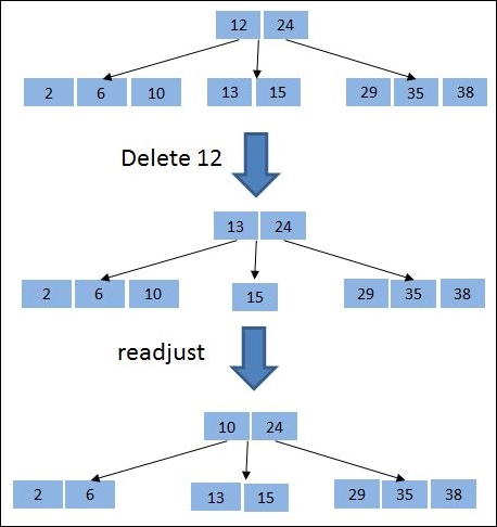
Figure 7.15: Example of deletion in B-tree
Queries are executed quickly if the data is stored in a sorted order as a linear indexing strategy. Thus, they are very good for static data. However, when it comes to adding operations such as insertion and deletion, they are not good, as it requires rewriting the whole data. When it comes to dealing with stored datasets, B-trees are good in indexing data in external storage devices as they read data in blocks, although any insertion and deletion could potentially lead to a lot of empty space. B+ trees generalize the B-trees to address this issue by keeping all the values in the leaf and the internal nodes only contain the keys. All the leaves which store values are linked, and the internal nodes only help to guide the operations on the leaves. A B+ tree stores up to d references to children and up to d-1 keys. An example of a B+ tree is shown in Figure 7.16:

Figure 7.16: Example of B+ tree
The B+ tree requires all leaves to be equidistant from the root node. Thus, in the example shown in Figure 7.16, searching for any value will require three nodes to be loaded from the disk - root node, second-level, and a leaf. In practice, depth d will be a number as large as it takes to fill the block in the disk. For example, if a block size is 6 KB, our block is an 8-byte integer, and each reference is a 4-byte offset, then d is selected as the maximum value by using the equation 8(d-1) + 4d ≤ 8192, which comes out to be 682. The following properties need to be maintained in a B+ tree:
- If a node has more than one reference, then it has keys.
- All leaves are at the same distance from the root node.
- Every Nth non-leaf node has k number of keys. All keys in the first child's subtree are less than N's first key, and all keys in the ith child's subtree (2 ≤ i ≤ k) are between the (i − 1)th key of n and the ith key of n.
- The root has a minimum of two children.
- Every non-leaf, non-root node has children between floor(d/2) and d.
- Each leaf contains at least floor(d/2) keys.
- Every key from the table appears in a leaf in a left-to-right sorted order.
The pseudocode for a B+ tree node using R is shown as follows:
bplusnode<-function(node=NULL, key, val){
  node <- new.env(hash = FALSE, parent = emptyenv())
  node$keys<-keys
  node$child<-NULL
  node$isleaf<-NULL
  node$d<-NULL
  class(node) <- "bplustree"
  return(node)
}
The child node is of type doubly linked list to have a connection as shown in Figure 7.11:
dlinkchildNode <- function(val, prevnode=NULL, node=NULL) {
  llist <- new.env(parent=create_emptyenv())
  llist$prevnode <- prevnode
  llist$element <- val
  llist$nextnode <- node
  class(llist) <- " dlinkchildNode"
  llist
}
The above function can be utilized to create a doubly linked list. In the case of a new object, a new environment is created as shown below while adding a value 1 to a new doubly linked list:

The B+ tree uses the copy-up and push-up approach for insertion. Let's take an example: Initially, B+ tree will have a single node during tree creation, and as the node overflows, the B+ tree will split the node into two. The new node is generated as the new root. The first key in the right node is copied up to the new root, as shown in Figure 7.17:
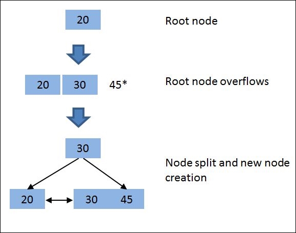
Figure 7.17: Example of B+ tree creation
The preceding example can be used to set up the insertion process for a B+ tree, which follows a schema very similar to the 2-3 tree insertion, and is stated in the following steps:
- Insert a key at the root if the node is empty
- If the node is full, then split the node into two, distributing the keys evenly between the two nodes
- For the leaf node, copy the minimum value in the second of these two nodes, and recursively repeat this to insert it into the parent node
- For the internal node, exclude the middle value during the split, and repeat the insertion algorithm to insert this excluded value in the parent node
Similar to the B-tree, the B+ tree supports exact match queries, that is, it finds the value for the given key. Furthermore, B+ trees are also very efficient for range queries, that is, finding all the values within a defined range. For an exact match query, the B+ tree follows a single path from the root node to leaf node, as depicted in Figure 7.18, which shows the search path for key 56:

Figure 7.18: Exact query match example in B+ tree
B+ trees also very efficiently support range queries, that is, finding all the objects within a defined range. This is due to the fact that all the leaf nodes are sorted and linked together. If we want to search for all objects lying within a defined range of values, this can be achieved by performing an exact match for the lower-value key, and then following the sibling leaf using connection. An example of a range query is shown in Figure 7.19:

Figure 7.19: Range query example in B+ tree
The preceding diagram shows an example of a range query for all objects between [56, 97]. The B+ tree first locates the lowest value within the tree, and then transverses through the nodes to find all the values till 97. The pseudo script in R for a range query is written as follows:
### Function for range queries
querry_search<-function(node, key1, Key2){
  ## Function to get values within leaf node using link list
  search_range<-function(child, key1, key2, val=NULL){
    if(child$element>key1 & child$key2){
      val<-c(val, child$element)
      search_range(child$nextnode, key1, key2, val)
    } else
    {
      return(val)
    }
  }

  if(key1>key2){
    temp<-Key2
    key2<-key1
    key1<-temp
  }
  child<-search_lower_key(node, key1)   # search lower leaf
  rangeVal<-search_range(child, key1, key2)   # Return Range
  return(rangeVal)
}
The search_lower_key function uses a structure similar to the search_key function in 2-3 node. Once the leaf with the lower key is identified, the search_range function transverses through the interconnected leaves to find all the values till the higher limit is hit.
To delete an object from a B+ tree, the path from the root to the leaf is identified, and then the object is removed from the leaf. After removal, if the leaf is more than half-full, then nothing needs to be done. However, if, after removal, the leaf size decreases to less than half, then the algorithm redistributes values from the neighbors to underflowing nodes. In cases where redistribution is not possible, the underflowing node is merged with a neighbor. An example of deletion is shown in Figure 7.20:

Figure 7.20: Deletion in B+ tree when leaf has sufficient number of objects after deletion
In Figure 7.19, the deletion of key 68 has not unbalanced the tree. However, if another element 67 is deleted from the tree, the tree readjusts as shown in Figure 7.21, and 79 is pushed up the node:

Figure 7.21: Deletion in B+ tree when leaf has an insufficient number of objects after deletion
In cases where neighboring nodes are not able to satisfy, then the nodes are merged and readjusted accordingly.
The B+ tree also supports standard of aggregation queries due to its efficiency with range queries such as count, sum, min, max, average, and so on. One approach to performing aggregation queries using a B+ tree is to keep a temporary aggregate value; starting with an initial default value, the aggregator keeps updating with every value found in the tree. On completion of the search, the aggregator's final value is returned. However, this approach is not efficient as it will require a computational effort of O(logb n + t/b), where t is number of keys and b is the tree average branching factor. The approach is also not suitable for large queries, as it requires a lot of disk pages to be accessed while aggregation. Another way to implement the B+ tree with reduced computation while aggregation is to store the aggregated values of the subtrees. Thus, when any query is executed, the local aggregates are used, and it avoids browsing the whole subtree.
B+ trees have received a lot of attention, and have been used widely in databases for indexing. Before we get into an analysis of the B+ tree, let's introduce some of its practical aspects. The minimum number of occupancy in B+ tree is 100. Thus, the fan-out parameter for a B+ tree will be between 100 and 200. From a practical perspective, an average page capacity in a B+ tree is around 66.7%.
Thus, a page with a fan-out parameter of 200 will contain 200*0.667 = 133 elements. Thus, the relationship between the height and the number of objects that a typical B+ tree can hold can be evaluated as shown in Table 7.1:

Table 7.1: Deletion in B+ tree when leaf has an insufficient number of objects after deletion
The initial levels of a B+ tree have very few number of pages. For example, if a disk page is 4 KB large, then the first two levels will hold 4*134=536 KB space on the disk, which is small enough to be stored in-memory, and need to be scanned to go down the leaf while searching.
In B-trees and B+ trees, operations are asymptotic with I/O cost of O(logb n), where n is the total number of records in the tree and base b is the tree average branching factor. The operation time for insertion, deletion, and search is the same in both B-trees and B+ trees as both data structures follow the path from the root to the leaf for an operation. Let's assume that the time spent on each node is O(d) in the main memory. As B-tree ensures every node is at least half-full, the average branching factor will be d/2 where d is the order. Thus, operations in a B+ tree are asymptotic with O(logd/2 n). The search, insert, and delete operations will take O(d logd/2 n) time. To further reduce the computation, especially while inserting a lot of records, the B+ tree uses bulk load approaches, which sorts in the input, and fills the leaf nodes in a sequential order in block of page size. If the keys are sorted, then the bulk load method reduces the insertion time by O(n/S), where 2S is the number of keys stored in a leaf.