System runtime is essential for benchmarking different algorithms. The process helps us to compare different options, and to pick the best algorithm. Benchmarking of different algorithms will be dealt with in detail in subsequent chapters.

The microbenchmark package on CRAN is used to evaluate the runtime of any expression/function/code at an accuracy of a sub-millisecond. It is an accurate replacement to the system.time() function. Also, all the evaluations are performed in C code to minimize any overhead. The following methods are used to measure the time elapsed:

In our current example, we will be using the mtcars data, which is in the package datasets. This data is obtained from 1974 Motor Trend US magazine, which comprises of fuel consumption comparison along with 10 automobile designs and the performance of 32 automobiles (1973-74 models).

Now, we would like to perform an operation in which a specific numeric attribute (miles per gallon (mpg) needs to be averaged to the corresponding unique values in an integer attribute (carb means no of carburetors). This can be performed using multiple ways such as aggregate, group_by, by, split, ddply(plyr), tapply, data.table, dplyr, sqldf, dplyr and so on. For illustration, we have used the following four ways:

Then, microbenchmark is used to determine the performance of each of the four ways mentioned in the preceding list. Here, we will be evaluating each expression 100 times.

> library(microbenchmark)
> MB_res <- microbenchmark(
+  Aggregate_func=aggregate(mpg~carb,data=mtcars,mean),
+  Ddply_func=ddply( mtcars, .(carb),function(x) mean(x$mpg)),
+  Data_table_func = mtcars_tb[,mean(mpg),by=carb],
+  Group_by_func = summarize(group_by(mtcars, carb), mean(mpg)),
+  times=1000
+ )

The output table is as follows:

The output plot demonstrating distribution of execution time from each approach is shown in Figure 2.4:

> library(ggplot2)
> autoplot(MB_res)

Figure 2.4: Distribution of time (microseconds) for 1000 iterations in each type of aggregate operation

Among these four expressions and for the given dataset, data.table has performed effectively in less possible time as compared to the others. However, expressions need to be tested under scenarios with a high number of observations, high number of attributes, and prior to finalizing the best operator.

Based on the performance in terms of system runtime, a code can be classified under best, worst or average category for a particular algorithm. Let's consider a sorting algorithm to understand this in detail. A sorting algorithm is used to arrange a numeric vector in an ascending order, wherein the output vector should have the smallest number as its first element and largest number as its last element with intermediate elements in subsequent increasing order. Currently, we will be implementing insertion sorting, however Chapter 5, Sorting Algorithms, will cover various types of sorting algorithms in detail. In insertion sorting algorithm, the elements within a vector are arranged based on moving positions. The best, worst and average cases are data dependent. Now, let's define best, worst and average case scenarios for insertion sorting algorithm.

Generally, the best-case scenarios are not considered to benchmark an algorithm, since it evaluates an algorithm most optimistically. However, if the probability of occurrence of best case is high, then algorithms can be compared using the best-case scenarios. Similar to best-case, worst-case scenarios evaluate the algorithm most pessimistically. It is only used to benchmark algorithms which are used in real-time applications, such as railway network controls, air traffic controls, and the like. Sometimes, when we are not aware of input data distributions, it is safe to assess the performance of the algorithm based on the worst-case scenario.

Most of the time, average-case scenario is used as a representative measure of algorithm's performance; however, this is valid only when we are aware of the input data distribution. Average-case scenarios may not evaluate the algorithm properly if the distribution of input data is skewed. In the case of sorting, if most of the input vectors are arranged in descending order, the average-case scenario may not be the best form of evaluating the algorithm.

In a nutshell, realtime application scenarios, along with input data distribution, are major criterions to analyze the algorithms based on best, worst, and average cases.

This section primarily deals with details on the trade-off between a computer's configuration and an algorithm's runtime. Let's consider two computers A and B, with B being 10 times faster than A, along with an algorithm whose system runtime is around 60 minutes in computer A for a dataframe of 100,000 observations. The functional form of algorithm's system runtime is n^3*. However, this functional form can be considered as an equivalent to the growth in the number of operations required to complete the running of the algorithm. In other words, the functional form of system runtime and the growth rate is same. The following situations will help us understand the trade-off in detail:

Situation 1: Will computer B, which is ten times faster than computer A, be able to reduce the system runtime of the algorithm to six minutes from the current 60 minutes?

This is perhaps yes, provided the size of the dataset remains consistent in both computers A and B. However, if we increase the size of the dataframe by 10 times, the following situation arises.

Situation 2: Will the algorithm in computer B be able to run the increased dataframe of 1,000,000 observations in 60 minutes, as computer B is 10 times faster than computer A?

This becomes tricky, as we are dealing not only with a change in computer configuration but also change in the size of input data, which makes the algorithm perform non-linearly (in our case-cubic form). The following table elucidates the capacity of computer B, which is 10 times faster than computer A, to handle the increase in size of the input dataframe, which can be run in a fixed time period for a given functional form of the algorithm's growth rate. Assume that computer A can perform 100,000 operations in 60 minutes, whereas computer B can perform 1,000,000 operations in 60 minutes. The *k is a constant positive real number ∼ same time period of x minutes for computer A and computer B.

 Figure 2.5: Performance comparison of widely used growth rate functions using two different sizes of dataframes

Let's understand each functional form of algorithm's growth rate:

Now, let's dive deep into situation 3, which deals with comparing the trade-off between algorithms and computers.

Situation 3: Which scenario is better for an algorithm with a growth rate functional form of n³- to increase the computer's performance capability,or to reconfigure the algorithm to change its growth rate functional form?

As we have already assessed the scenario of increasing the system's performance capability under Situation 2, let's now try to analyze the situation of reconfiguring the algorithm's growth rate functional form.

Currently, our algorithm possesses a functional form of n³. For an input data of size 1,000, the total number of operations required is 1,000³. Suppose, if the current algorithm can be reconfigured to nLog₁₀(n), then the total number of operations would reduce to 3,000, which is much lower than 1,000³. As the number of operations using n³ is more than 10 times the number of operations using nLog₁₀(n) for every n>2, it is more advisable to reconfigure the growth functional form of the algorithm rather than increase the computational performance capability by 10 times.

To summarize the trade-off:

As we learned earlier, an algorithm is a step by step procedure designed to analyze and compute a given problem in a language understandable by a computer. Asymptotic analysis of an algorithm is a mathematical representation to determine its runtime performance or growth rate with the necessary boundary conditions. The boundary conditions depend on factors such as computer configurations, growth in the size of input data, coefficient of the growth rate function (also referred to as constant (k) in section Computer versus algorithm), and others. However, the capability to handle larger data sets is more dependent on the increment in computational performance of computers rather than on the constant term in the growth rate functional form. Also, the curves of different growth rate functional forms do intersect irrespective of the value of the constant in those equations. Thus, the constants in the growth rate or system runtime functional forms are generally ignored while comparing performances at computer level or at the algorithm level. Nevertheless, it is desirable to consider constants in the following situations:

Asymptotic analysis is also used to determine the best, worst, and average case of an algorithm, as it is a function of input size which evaluates the runtime of the algorithm. For example, the performance of a sorting algorithm can be evaluated using the incremental length of input vectors. The following are asymptotic functions for standard insertion sorting and merge sorting:

In the preceding two functions, α and c are constants and n is the length of the input vector.

One needs to bear in mind that asymptotic analysis provides only a ballpark estimation of the algorithm's performance in terms of system runtime consumption.

The following asymptotic notations are commonly used to determine the complexity in calculating the runtime of an algorithm.

Upper bounds or Big O notation

The upper bound of an algorithm's running time is denoted as O. It is used in evaluating worst-case scenarios, and determines the longest running time for any given length of an input vector. In other words, it is the maximum growth rate of an algorithm.

Figure 2.6: f(n) is Big O of g(n) for all n>k

Let us consider two functions, f and g, which determine an algorithm's runtime t based on varying input vector length n. These functional forms f(n) and g(n) should be non-negative or non-decreasing, because as the length of the input vector increases, the running time of the algorithm practically increases. These functional forms are equivalent to the running time of best, average, and worst-case scenarios of any given algorithm.

As we can see, initially c*g(n) is lower than f(n) for values of n<k, and subsequently, c*g(n) is higher than f(n) for n>k. Thus, the upper bound of the algorithm can be represented as follows:

f(n) = O(g(n)) that is-f(n) < c*g(n) for n>k>0 and c>0.

Therefore an algorithm with a growth rate f(n) is known as Big O of g(n) only when f(n) executes faster than g(n) for all possible inputs n (n>k>0) and any constant c (c>0).

Now, let's consider an algorithm whose running time can be expressed as f(n) of polynomial order 2, and we need to determine g(n), which represents the upper bound for f(n):

f(n) = 25 + 12n + 32n²+ 4*log(n)

Now, for every n>0:

f(n) < 25 n² + 12 n² + 32n²+ 4 n²

f(n) < (25+ 12+ 32+ 4)n²

f(n) = O(n²), wherein g(n) is n² and c=(25+12+32+4)

However, there exists a limitation with this approach. If the coefficient of the linear function is very high, then a polynomial of higher order or an exponential with a smaller coefficient is preferred in practical scenarios.

The following are some of the growth orders widely used to assess an algorithm's performance. Both 2^O(n) and O(2ⁿ) yield different results and different interpretations as shown in the following figure:

 Figure 2.7: Big O representation of various growth order functions

Lower bounds or Big Omega notation (Ω)

The lower bound of an algorithm's running time is denoted as Ω. It is used in evaluating the least running time of an algorithm, or the best-case scenario for any given length of input vector. In other words, it is the minimum growth rate of an algorithm.

 Figure 2.8: f(n) is Big- Ω of g(n) for all n>k

Let us consider two non-negative and non-decreasing functions f(n) and g(n), which determine an algorithm's runtime t based on a varying input vector length n. These functional forms are an equivalent to the running time of best, average, and worst-case scenarios of any given algorithm.

As we can see, initially c*g(n) is higher than f(n) for values of n<k, and subsequently, c*g(n) becomes lower than f(n) for n>k. Thus, the lower bound of the algorithm can be represented as follows:

f(n) = Ω (g(n)) that is-f(n) > c*g(n) for n>k>0 and c>0.

Hence an algorithm with growth rate f(n) is known as Big O of g(n) only when f(n) executes faster than g(n) for all possible input n (n>k>0) and any constant c (c>0).

Now, let's consider an algorithm whose running time can be expressed as f(n) of polynomial order 2, and we need to determine g(n), which represents the lower bound for f(n):

f(n) = 25 + 12n + 32n²+ 4*log(n)

Now for every n>0, the largest of the lower bound is as follows:

f(n) > 25 n²

f(n) > Ω (n²) wherein g(n) is n² and c=25

The smallest of lower bound is as follows:

f(n) > 25

f(n) > Ω (25)

Here, g(n) is a constant and c=25.

Big θ notation

As you just learned, about O and Ω, which describe the upper (maximum) and lower (minimum) bound of an algorithm's running time respectively, θ is used to determine both the upper and lower bound of the algorithm's runtime, using the same function. In other words, it is asymptotically tight bound on the running time. Asymptotically because it is significant only for large number of observations, and tight bound because the running time is within constant factor bounds:

 Figure 2.9: f(n) is Big- θ of g(n) for all n>k

Let us consider two non-negative and non-decreasing functions f(n) and g(n) which determine an algorithm's run time t based on varying input vector length n.

Then, for every n>k>0 and c>0,

f(n) = θ(g(n)) if and only if O(g(n)) = Ω (g(n)).

Simplifying rules

Big O (upper bound), Big Omega (lower bound), and Big Theta (average) are the simplest forms of functional equations, which represent an algorithm's growth rate or its system runtime. Simplifying rules can be used to determine these simplest forms without worrying much about formal asymptotic analysis. These rules are applicable to all the three simplest forms. However, the examples shown in the following table are based on the Big O asymptote.

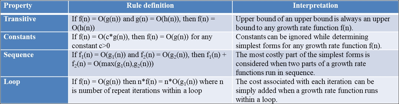
 Figure 2.10: Definition of simplifying rules along with their interpretations

These simplifying rules are widely used in the following chapters while evaluating costs for an algorithm's growth rate or system runtime functional form.

Classifying rules

Let's consider two algebraic growth rate functions f(n) and g(n). The classifying rules are then used to determine which functional form has a better performance over the other. This can be evaluated using the limit theorem, which is as follows:

The following three scenarios are used to classify f(n) and g(n):

Figure 2.11: Classifying rule forms

Let's' evaluate the computations of different components within a program or algorithm using asymptotic analysis.

int_Vector <- 0:60

Component 2 - Simple loop

Consider a simple for loop with assignment operations.

a <- 0
for(i in 1:n)
a <- a + i

The following are asymptotes for each line of execution in the code:

Figure 2.12: Asymptotic analysis of a simple for loop

Hence, the total cost of this for loop using simplifying rules is θ(n).

Component 3 - Complex loop

Consider a complex loop using a while loop, and a nested for loop using assignment operations.

a <- 1
i <- 1
b <- list()
while(i<=n )
{
  a <- a + i
i<- i+1
}
for(j in 1:i)
for(k in 1:i)
{
  b[[j]] <- a+j*k
}

The following are asymptotes for each line of execution in the code:

Figure 2.13: Asymptotic analysis of a complex loop

Hence, the total cost of this complex loop using simplifying rules is θ(n²).

Component 4 - Loops with conditional statements

Consider a for loop with a nested if...else condition, as shown in the following example code:

a <- 1
for(i in 1:n)
{
  if(i <= n/2)
{
for(j in 1:i)
a <- a+i
}else{
a <- a*i
}
}

The following are the asymptotes for each line of execution in the code:

Figure 2.14: Asymptotic analysis of a conditional loop

The total cost of this loop with if...else conditions using simplifying rules is θ(n²). The cost assessment of an if...else condition is evaluated using the worst-case scenario. Here, the worst-case scenario is when the if condition is True, and the nested for loop is executed instead of a simple for loop in the else condition. Hence, maximum growth rate (or system runtime) is considered for evaluating the asymptote of the conditional statements.

Component 5 - Recursive statements

A statement which iterates in a loop using the same function till a condition is satisfied is called a recursive statement. The most commonly used recursive statement is the factorial function. The following code calculates the factorial of an integer n.

fact_n <- 1
for(i in 2:n)
{
  fact_n <- fact_n * i
}

The following are the asymptotes for each line of execution in the code:

Figure 2.15: Asymptotic analysis of a recursive statement

The total cost of a recursive statement using simplifying rules is θ(n).

Algorithms form an intrinsic base for analyzing a problem, and each problem can be analyzed using multiple algorithms. These algorithms are further evaluated based on their functional performances, as covered under previous sections. However, there arises a basic question-how to evaluate a problem which has many solutions vis-à-vis many algorithms.

Consider a problem with m number of algorithms, where m tends to infinity. Then, the upper bound or the worst-case scenario cannot be lower than the upper bound of the best algorithm, and the lower bound or the best-case scenario cannot be higher than the lower bound of the worst algorithm. In other words, it is easier to define the lower and upper bounds for an algorithm, but it becomes tricky when it is to be defined for a problem, since there might be algorithms which might not have been explored at all.

More details along with examples will be covered in subsequent chapters.

So far, the performance of an algorithm was evaluated using only its functional form of system runtime. Another functional form can be a key constraint for algorithm developers in system space or available memory. The space functional form depends on both the type and size of data structure unlike the runtime functional form, which depends primarily on the size of the input data structure. As an example, a vector of n elements requires k*n (θ(n)) bytes of memory provided that each element requires k bytes. The space required by each data structure depends on the mode of data storage for efficient data access within.

For example, a linked list not only stores a list of elements but also pointers for easy navigation within. These pointers are additional storage elements, which act as overheads and require additional space allocation. Thus, a data structure with lower overheads can enhance the performance of algorithms in terms of space functional form.

However, there needs to be a trade-off between the system's runtime and space requirement for effective evaluation of an algorithm. The best algorithm is one which requires less space and less runtime. But in reality, satisfying both criteria is difficult for algorithm developers. In order to reduce space requirement, developers tend to encode data information, which, in turn, requires additional time to decode, thereby increasing the system runtime. On the other hand, developers tend to restructure data storage information while executing algorithms to decrease the system runtime at the expense of greater space.

More details along with examples will be covered in subsequent chapters.