Chapter 9: Software-Defined Radio Attacks

Modern embedded devices communicate a lot over radio interfaces in order to be independent of cables. It is very common for them to use the well-established protocols (such as Wi-Fi or Bluetooth) that we already looked into in previous chapters. There are numerous systems that don't need such complex protocols (or are constrained due to other design considerations, such as cost, complexity, processing power, and more) but still have a need for radio communications. In this case, they tend to use other protocols that are not necessarily easy to interface with out of the box. In this case, we need to be able to interact with these custom protocols in order to be able to test the communication's security. This is the domain of Software-Defined Radio (SDR).

We will go over the following topics in this chapter:

• Introduction to arbitrary radio/SDR
• Understanding and selecting the hardware
• Looking into the radio spectrum
• Finding back the data
• Identifying modulations
• Demodulating the signal
• Sending it back

Technical requirements

You will need at least an SDR adapter. The bare minimum hardware requirement is an RTLSDR stick that I will talk about in the next section. You will also need the following software tools:

• GNU Radio
• Gqrx
• baudline
• Audacity
• Python

Check out the following link to see the Code in Action video:

https://bit.ly/3uKVsRz

Introduction to arbitrary radio/SDR

SDR allows you to receive (and emit if you have the adequate license and hardware) arbitrary radio signals. The adapter acts as a device that can sample (some can also emit) radio signals around a frequency you can specify and that is it. All the signal processing is done on the software. The theoretical aspects of the sampling and how the samples represent the radio data is a little complicated; it is not absolutely necessary to understand it to start but it will become very useful later when you start to develop your own scripts and signal processing chains in GNU Radio.

Note

To understand the theoretical principles of SDR and basic usage of GNU Radio, I strongly advise looking at this excellent series of videos by Michael Ossman: https://greatscottgadgets.com/sdr/1/.

Understanding and selecting the hardware

As usual, the hardware capabilities and costs are linked. Here is a list of the main domains that the hardware selection impacts, with a list of the main SDR adapters and their capabilities per domain.

The hardware will mainly define the following:

• The frequencies you can access are as follows:

  - RTL-SDR (receive only): 20 MHz–1.75 GHz

  - HackRF: 10 MHz–6 GHz

  - BladeRF: 300 MHz–3.8 GHz

  - USRP: 70 MHz–6 GHz

• The width of the spectrum you can cover in one shot is as follows (the sample rate in MS/s is the number of samples it takes per second. It is also the width of the spectrum that is captured):

  - RTL-SDR: 2.4 MS/s

  - HackRF: 20 MS/s

  - BladeRF: 40 MS/s

  - USRPs: 61 MS/s

  The higher the sample rate you have, the faster you can explore the spectrum, but it will (most of the time) not impact your capability to analyze signals since most of the signals have a bandwidth of a few dozens of KHz in the lower frequencies.

• The price range is as follows:

  - RTL-SDR: ~25€

  - HackRF: ~300€

  - BladeRF: ~400€

  - USRPs: ~1,000€+

Once you have decided on your hardware, let's use it to look into a radio device.

Looking into a radio device

First, get yourself one of the multiple radio-emitting simple gadgets that are currently on the market (such as a garage opener or a radio-commanded relay box) and see whether information is available in the FCC documentation (https://www.fcc.gov/oet/ea/fccid or https://fccid.io/). Since the Furby does not use radio, I'll look into an IKEA radio-controlled LED lighting device (ANSLUTA). There is no apparent FCC number on the emitter or receiver, but a simple internet search lends the FCC ID as FHO-E1205. Opening the emitter (using the same approach we used in previous chapters) shows a TI CC 2500 chip. Looking into the CC2500 documentation, we can see that the frequency should be ~2.45 GHz (2.4–2.48 from the CC2500 datasheet: https://www.ti.com/lit/gpn/cc2500) and this is confirmed by the FCC documentation.

If you are using an RTL-SDR, this frequency will be out of your reach. Pick a wireless garage door opener in the lower ISM bands (433 MHz–800 MHz, depending on where you live). The principles will be the same.

Receiving the signal – a look at antennas

When looking into an antenna to receive your signal, there will be two cases:

• The device emits on a frequency for which commercial antennas are available. Just buy an antenna; you can reuse it later and it will be nicely designed, and you won't have to worry.
• The device emits on a frequency for which commercial antennas are not available. Most of the time, we will be working quite close to the device we will be testing. That means we won't need a very performant antenna to be able to receive the signal, but we will need something that works at least half-decently in our target band.

  Antenna design could cover two or three books on its own (it is a very complex domain on its own), their pros and cons too (look into antenna books on your favorite bookseller's website if you want confirmation). For our usage, we can just use simple, throwaway dipole antennas that I stick to a length of PVC tube, or buy a ready-made antenna that matches our frequency range of interest.

Now, let's look at what to do when you don't have a commercial antenna.

Making a quick and dirty dipole antenna

The dipole antenna is very simple. It is two lengths of wire forming an antenna of a fractional length of the signal wavelength.

Usually, half-wavelength works great (but 1/4, 1/8, and more can be used if 1/2 is too big). The wavelength is C x (1/(Frequency)).

Let's imagine something emitting at 520 MHz (in my country, that can be medical devices, radio microphones on onboard vehicular communication, and so on).

Now, let's calculate the antenna parameters for 520 MHz:

Next, we build the antenna by measuring two adequate lengths of wire for the target frequency (for a half-wave, measure two quarter wavelengths, for a quarter-length, measure two eighths, and so on).

For a half-wave 520 MHz antenna, that is 2 x 14.4 mm.

In the following figure, we can see how the wires are connected to the SDR device:

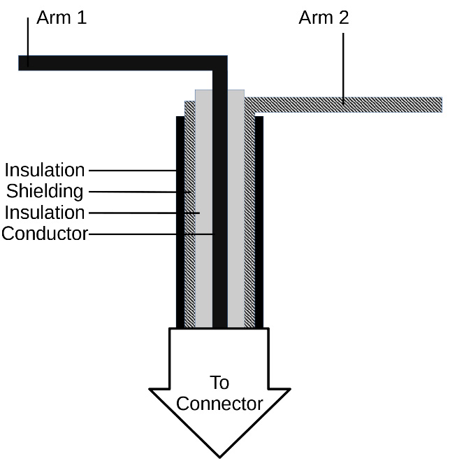
Figure 9.1 – Dipole antenna connection

This should be enough for correct reception. Just keep in mind that the dipole antenna is unbalanced; you should (it helps but is not mandatory) use a balun (balanced/unbalanced) right before the dipole in order to balance it (to overly simplify, it avoids unwanted currents coming into your receiver and correctly references the signal). Either buy one that fits your transmission line impedance (depends on your coax type and length) or make an air-choke by making a coil of a few turns of your coax (this is a bit more complicated to do but is basically free; it requires you to measure the capacitance to determine the correct length of coax to coil up). To do so, look into this: https://www.instructables.com/id/Air-Choke-Ugly-Balun-for-Ham-Radio/.

Here is the (not) very fancy 75 cm/branch half-wavelength antenna I use for 100 MHz:

Figure 9.2 – Antennas don't have to be fancy to work

This uses an ugly 3D-printed balun from http://www.dk0tu.de/users/DB4UM/c3d1pole/.

Looking into the radio spectrum

Gqrx is a GNU Radio application that allows you to have a nice GUI to set the frequency of your hardware and have a visual representation of the radio spectrum around the set frequency. It also allows you to hear some common modulations, such as narrow- or wide-band FM (WFM), lower and upper side band (LSB and USB), and others.

Let's fire up Gqrx and set up the source (hackrf for hackrf, RTLSDR for RTLSDR, and so on):

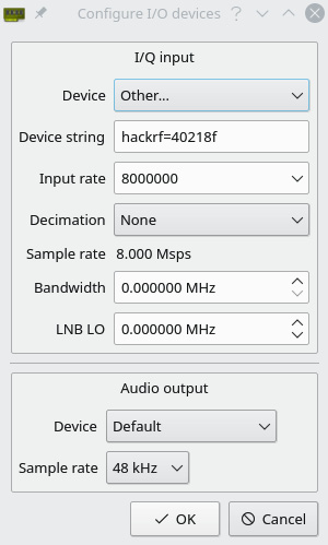
Figure 9.3 – Selecting the source: a HackRF example

The following screenshot shows the Gqrx main window:

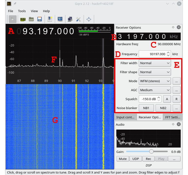
Figure 9.4 – Gqrx main window

The frequency you are listening to is as follows:

• A: The frequency you are listening to
• B: The frequency delta between the hardware-centering frequency and the part of the captured data the software processing is focusing on
• C: The frequency the hardware is centered on (that is, the frequency it will be capturing data around)
• D: Same as A
• E: The signal processing chain that will be applied to the data (here, set up to listen to (W)FM radio)
• F: The FFT scope
• G: The cascade scope (that is, the history of the FFT scope that flows down like a cascade)

Now, let's have a look at ~90 MHz. Normally, you can see two subwindows: a top one (the FFT) and a bottom one (the cascade) where you see peaks at frequencies that are emitting signals in the FFT and the history of these peaks in the cascade. Set the mode to WFM (right side of the GUI) and move the cursor to one of these peaks. You should now hear music (such as songs or someone speaking)! Wonderful, this is your first SDR use!

Now, look at the FFT plot in the following figure and you can see you have a big, thin peak right in the middle. This is your hardware center frequency (the big peak at 2.429 GHz in the following example). This peak comes from the hardware and cannot be removed. It would pollute your signals and that is the reason why you always have a shift next to the center frequency (the vertical line at 2.4355 GHz in the following figure) to listen to a specific frequency.

If we move to 2.45 GHz (go on the frequency and use your mouse wheel), we can have a look at our radio controller (not shown in the figure for clarity purposes). Here, our main problem is that the portion of the spectrum we are looking at (2.45 GHz) is pretty crowded (it's an ISM band after all; plenty of devices (including Wi-Fi) are emitting there):

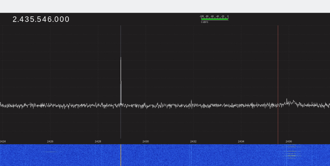
Figure 9.5 – FFT and cascade plots in Gqrx

So, let's go from 2.4 to 2.48 GHz by a step of our 1/2 sample rate and click on the device to see it emitting.

I find that mine is emitting around 2.436 GHz. Can you see the horizontal lines in the cascade? These are radio pulses you see when you click the remote control buttons.

Finding back the data

GNU Radio is a set of software tools that allows you to create a signal processing chain for the data that comes from your SDR hardware (or a file) to either your hardware again (to emit) or a file. The blocks in its GUI (gnuradio-companion) are individual processing steps in the signal processing chain. Data comes from a source toward a sink (both are files or your SDR hardware driver, your sound card, or... well, it can be a lot of things: another program, a network endpoint, and so on).

Note

gnuradio-companion (grc) has two main GUI frameworks it can talk to: QT and WX. Depending on your installation, you may have to change the framework in the generate options block. The GUI-related processing blocks will also have to be changed in the processing flow itself.

So, let's fire up gnuradio-companion and make a receiver.

First, let's replicate Gqrx and let's have an FFT visualization. FFT is a visualization of the signal in the frequency domain (that is, the strength of the different components as a function of their frequency).

Add a source (depending on your hardware, the osmocom source for hackrf, for example; right column, Ctrl + F to search) and an FFT sink (it can be named FFT or Frequency sink, depending on the version; for now, default values should be fine, just change your sample rate variable to the best your hardware can do) and link them (by drawing from the output of your source to the input of the FFT).

All .grc files describe a signal processing chain in GNU Radio and are available in the Git repository of the book. I will also provide a file with the samples that are coming from my receiver so that you can replicate these steps (you will need to replace the osmocom source with a file source pointing to the sample file).

Open fft.grc and run it:

Figure 9.6 – A typical FFT plot (here, centered on Wi-Fi frequencies)

Now, let's center on our emitting channel:

• Focus on it by reducing the sample rate (it removes signals from higher and lower frequencies) in the Osmocom source block.
• Add a low-pass filter, a width around what the signal you receive seems to be (it focuses even more sharply). This is the low-pass filter block.
• Add two scopes: one on our raw signal and one on our mag^2 (the square of the magnitude will make emissions "pop out"). These are the time sink blocks.

It should look like this:

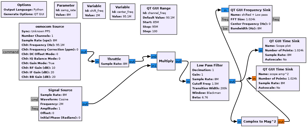
Figure 9.7 – Our flow graph with additional visualizations

Run it to see the size of the received samples on the time domain (use fft-scope.grc if you can't make it work on your own):

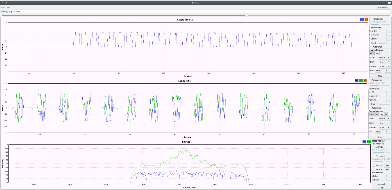
Figure 9.8 – Example of the three visualization flowgraphs

Here, we can see that the trains of magnitude (top scope) have the same width and spacing. If we zoom closer into one, it is not clear at this point whether it is a repeated signal, but they don't seem to contain clear on/off sequences inside. This is not on-off keying (OOK), and in the bottom FFT, we cannot see "spikes" that could indicate frequency shift keying (FSK). So now, what is the modulation?

Identifying modulations – a didactic example

What we now have is a very common question when looking into unknown signals: what is the modulation? Finding the correct modulation and parameters can require a bit of detective work, even if you know the parameters. This section is more of an illustration of the process of reversing a signal modulation than directly a recipe (since there is no recipe). Some people are currently working in an academic context on projects to train neural networks to do signal classification, meaning there is no straightforward way to recognize modulations.

In the case of the light controller, we can already reduce the candidate's number because we know (from the FCC documentation and opening the device) that it embeds a CC2500. The datasheet tells us that it supports a few modulation schemes: 2-FSK, GFSK, MSK, and OOK. We already eliminated two (OOK and FSK) but how do we tell the difference between them?

First, let's talk about what modulation is. Modulation is a way to transmit information in a radio signal. It can be digital (OOK, FSK, G-FSK) or analog (AM, FM, and more). Modulation is the way the information is "inserted" in the physical characteristics of the signal (changes in frequency, phase, amplitude, and others).

Second, let's talk about what modulation is not.

Modulation is not encoding. Encoding is the way to describe data, not the way data is inserted in the signal. Let's take an example with a very simple modulation: OOK. OOK is basically knowing whether a signal is on or off. Now, how can you encode data over OOK? You can do it in multiple ways, actually! Take the following examples:

• You can have long pulses for 0 and short for 1 (or vice versa).
• You can have data encoded in the transition of the modulation. For example, if a modulated signal changed in the symbol time slot from low to high, it's a 1, and if from high to low, it's a 0 (this is called Manchester encoding).
• You can use the length of the pause in between high pulses to encode the information.
• And others...

When looking into a signal, you will also have to understand how that data is encoded.

Here are a few common modulations (there are plenty of modulations), as well as a brief explanation of how they work and how to recognize them.

AM/ASK

The main points related to AM/ASK are as follows:

• Modulation: Amplitude modulation/amplitude OOK.
• Type: Analog/digital.
• How it works: The signal amplitude (for AM/ASK) or the fact that it is there or not (OOK) carries the information.
• How to recognize it in GNU Radio: In a scope view coming from a mag or a mag^2 block, we can see trains of data.

Visual examples of modulation (sending 1,0,0,0,1,1,0,1) are shown in the following figure:

Figure 9.9 – ASK modulation

Next, let's look at FM/FSK.

FM/FSK

The main points related to FM/FSK are as follows:

• Modulation: Frequency modulation/FSK.
• Type: Analog/digital.
• How it works: The carrier frequency is modulated to carry the information, going a little up or down to carry the information (for example, in FM radio, this is done in a continuous way (as opposed to a discrete way in FSK) to carry the sound frequency.
• How to recognize it in GNU Radio: In the FFT, for FSK, you will see two (or more; two spikes is 2-FSK, three is 3-FSK, and so on) peaks very close to each other when looking at the signal up close. For analog FM, the peak of the carrier frequency will be consistently wide.

Visual examples of modulation (sending 1,0,0,0,1,1,0,1) are shown in the following figure:

Figure 9.10 – FSK modulation

Next, let's look at PM/phase shift keying (PSK).

PM/PSK

The main points related to PM/PSK are as follows:

• Modulation: Phase modulation/phase shift keying.
• Type: Analog/digital.
• How it works: The phase of the carrier is shifted to carry the information.
• How to recognize it in GNU Radio: When you use a Complex to Mag phase block and output the results to a scope, you can see brutal changes in the signal phase.

Visual examples of modulation (sending 1,0,0,0,1,1,0,1) phase changes are hard to see in the signal itself, but see how the sine jumps:

Figure 9.11 – PSK modulation

Next, let's look at minimum shift keying (MSK).

MSK

The main points related to MSK are as follows:

• Modulation: Minimum shift keying.
• Type: Digital.
• How it works: The amplitude and phase of the carrier are shifted to carry the information.
• How to recognize it in GNU Radio: You will see both magnitudes and phase change in the output of a Complex to Mag phase block and quite often, the changes will be in sync. MSK acts on two variables (magnitude and phase) and transmits symbols instead of just bits.

Since MSK is very hard to see in the signal itself (phase jumping especially), here is an AM modulation also sending symbols so that you can understand the difference between a bit and a symbol better (sending 1,0,2,3,1,2,0,1):

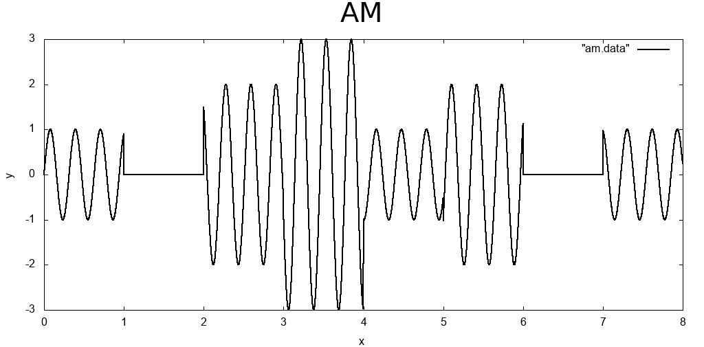
Figure 9.12 – AM modulation

Let's now learn how to get back our signal.

Getting back to our signal

So, what about our transmitter? We see trains of transmission on the magnitude scope but no obvious variation in length or rhythms in the train; it's not really looking like OOK. Within the pulses (the wagons in the train), we see some variations in amplitude but no real on/off. We don't see clear spikes in frequency, so it's not an x-FSK. The CC2500 datasheet (https://www.ti.com/lit/ds/swrs040c/swrs040c.pdf) leaves us with GFSK and MSK as possible modulations.

Let's look into the signal to see whether we can identify one of these two:

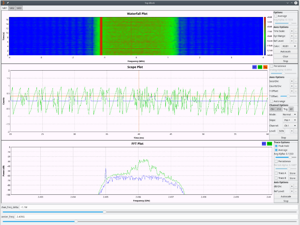
Figure 9.13 – Looking into the CC2500 signal

Let's look into GFSK. GFSK stands for Gaussian FSK; it is basically the same as FSK with a filter that ensures a smooth transition between the frequencies, hiding the very clear spikes we can see in simple FSK (in the preceding figure: FFT plot/waterfall plot).

MSK is using both amplitude and phase to carry the information and we don't see multiple "heights" in the trains that were output by the Mag^2 block (in the scope plot).

It doesn't show something that would contradict it being GFSK.

Demodulating the signal

At this point, GFSK and MSK are still possible candidates (since we had amplitude variations in the pulses). Let's adjust our filtering to just see the signal. Add a file sink to your GNU Radio flowgraph (grab a file sync block in the GUI and route the output of the final block to the input of the file sink; the filename is in the file sink block options) and capture an emission.

Open your output file in Audacity (File | Import | Raw data | 32-bit float) and adjust your sample rate to the one you used in your flowgraph. The file in Audacity looks as follows:

Figure 9.14 – Signal in Audacity

You can now trim the file to keep just the emission. Export it as Other uncompressed file | RAW headerless | 32bits float.

Now, let's work on this isolated sample to try to demodulate it.

GFSK is frequency-based, so if we try to demodulate the cut sample with a quadrature demod block, we should see something significant. Let's output it to a file sink after the quadrature demod (sampled-simpleqdemod.grc) and open it in baudline:

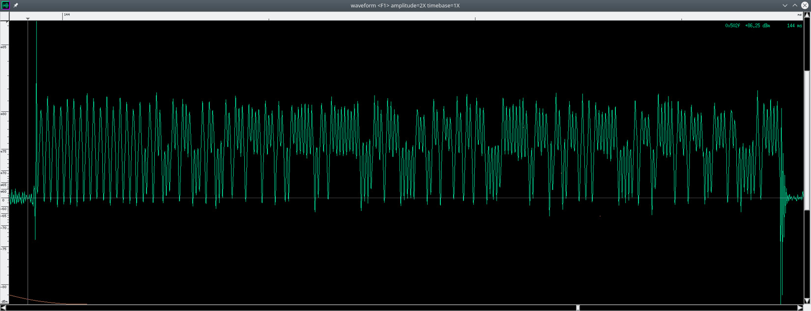
Figure 9.15 – Output of the attempted quadrature demod in baudline

Now we can see trains in the waveform window. We are going in the right direction. At this point, we have a little problem; we need to measure the time width that the smallest peaks take but the signal is so fast that baudline's ruler (on top of the waveform window) cannot go that low (it is graduated in milliseconds).

Well, we will then lie to baudline and load the file with a sample rate divided by 1,000. Let's say that I sampled the signal at 2 MS/s; that means that there are 2 million samples per second. If we load our file at 2 MS/s, it will appear 1,000 times slower in baudline, meaning that we can now use the ruler and replace the units with microseconds.

When we measure the fastest peaks (at the head of a train, they are called the preamble and are there to allow clock synchronization), we find that they are 8 µsec wide. As is, it would be 125 Kbauds, a data rate that is supported by the CC2500, which means we are still consistent! So now we have a good candidate for the baudrate. Let's refilter the demodulated signal (125e3 width and half of this in the cutoff; see sampled-simpleqdemod-refilterbds.grc).

It looks quite okay for the quadrature demodulation of a GFSK signal! Maybe it's still FSK but we didn't see the signal well in the FFT. When looking into an unknown signal, keep in mind that your assumptions are still assumptions; backtracking on them is not a bad thing. At this point, we don't really know whether it is GFSK or FSK. Let's keep in mind that the modulations are quite close (frequency with transition smoothing for GFSK; maybe we can get away with just treating it as FSK).

Here is how it looks in baudline:

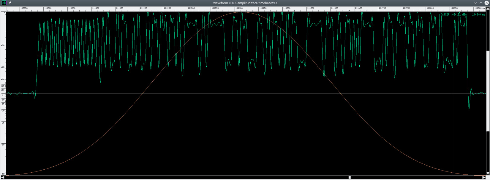
Figure 9.16 – Checking the baudrate in baudline

Now, let's center our signal (the train is not alternating around 0 and we need that to decode it). So, let's add an add const block in front of a scope sink in GNU Radio and let's center it around 0:

1. Enable the scope sink.
2. Disable the file sink.
3. Enable repeats in the file source in sampled-simpleqdemod-refilterbds.grc.

Here is the zero-centered signal (before, the bottom of the signal was at 0, while now the signal is alternating around 0):

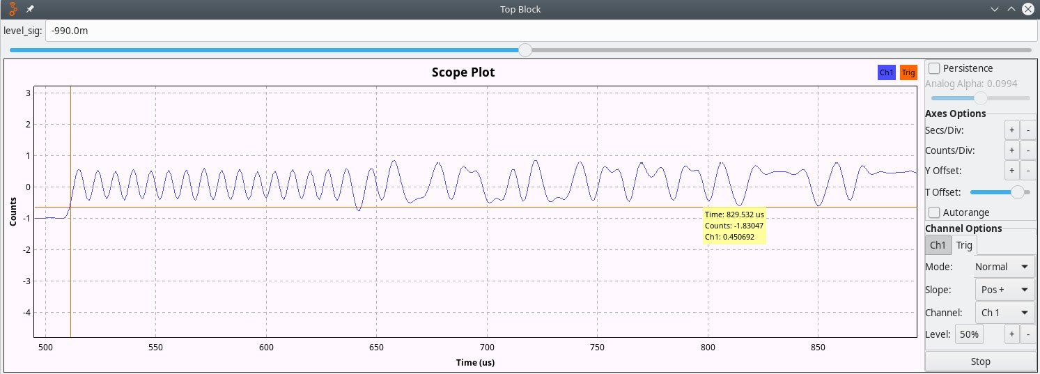
Figure 9.17 – Zero-centered signal

Now we need to use a Muller & Muller clock recovery block (Clock Recovery MM; the details are covered later in the chapter):

First, we need to know how many samples we have per symbol. I was sampling at 2 MS/s and the peak is 8 µsec: 2e6 * 9e-6 = 16 samples per symbol.

Let's bit-slice the output and sink it to a file. When we look into this file, we see that we indeed have output bits (1 byte per byte), but we don't see the preamble (usually 010101 or 101010)! We either did something wrong when processing the signal or one of our assumptions was bad. When we look back at the signal, we see that the preamble is looking just like sine, not regular pulses. This means that it is probably Manchester encoded! Do you remember Manchester encoding? The encoding is in the direction of the change.

One peak like that is 2.4 bits (to say almost 2.5 bits) in Manchester, so let's correct our baudrate to 125*2.4 = 300 Kbauds. Let's try this with our manual processing; let's add a GFSK block in parallel and plot it to see whether GNU Radio is doing a better job at this than us:

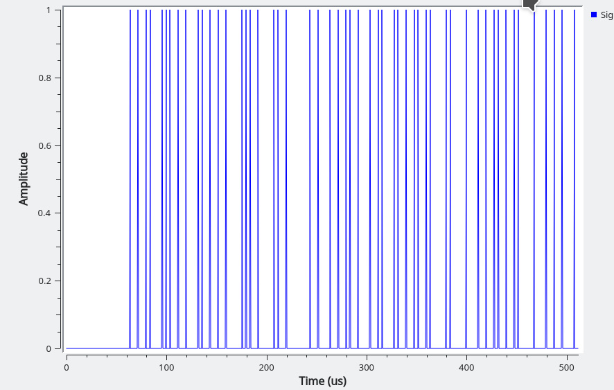
Figure 9.18 – Attempted demodulated signal

No dice, we don't get the preamble either, but when we look at the waveform, it is kind of unstable. There is something to it but there is definitely something wrong with the signal processing. Now, the waveform in the preceding screenshot is kind of looking like what I had when I was looking at the amplitude. I'll recapture the signal at a better sampling rate (10 MS/s) and look into OOK again.

When looking into it, actually the amplitude is looking more stable; was it OOK in the end and did I go on a wild goose chase? (Totally something that happens when I try to devise what modulation is in use.) If I do a complex to mag squared, with a line level correction a Clock Recovery MM, and reevaluate the baudrate ((10e6 * 9e-6)/2.5 = 36 samples per symbol, which is 277,777 bauds, which is possible but we'll try 40 samples per symbol too since humans like round numbers), then I really have something that looks like a preamble! It works at 40 samples per symbol!

This wild goose chase had the merit of allowing us to go through the different common modulations and to give us a leg up on how to identify a modulation!

Clock Recovery MM

Muller & Muller Clock Recovery is notoriously tricky to set up (and finicky; it is sensitive to signal level, for example). Let's have a look at the parameters and documentation of Clock Recovery MM:

• The documentation says the following:

  "The peak to peak input signal amplitude must be symmetrical about zero", " M&M timing error detector (TED) is a decision directed TED, and this block uses a symbol decision slicer referenced at zero."

  The signal must be centered on zero.

  "The input signal peak amplitude should be controlled to a consistent level (e.g. +/- 1.0) before this block to achieve consistent results for given gain settings; as the TED's output error signal is directly affected by the input amplitude."

  Signal conditioning for MM is very important. Signal normalization is crucial (we need to have a signal that is roughly symmetrical, without "big peaks").

• Omega (ω): Sample per symbol (that is, symbol rate), but it is an initial estimate. Clock Recovery MM is actually an adaptative filter; omega can and will change a little during the signal processing.
• Mu (µ): Initial phase. This is not important; it will change very rapidly internally, and we don't know the phase of the signal, so leave it at 0.
• Mu gain: The gain in the phase feedback loop.
• Omega gain: The gain in the frequency/sample per symbols feedback loop.
• Omega relative limit: The maximum variation of omega we want.

  Note

  Wow, this is a lot to digest. The original article (https://pdfs.semanticscholar.org/ef0a/539a61e05df52faeeeb8ca408e2f12575a8b.pdf) is a nightmare of mathematical formulas that needs a good day to read and another to reread and digest. It is a lot but I really encourage you to invest the time and effort.

So, is there something more practical for asynchronous analysis?

WPCR

Definitely! Let's have a look a Michael Ossmann's Whole Packet Clock Recovery (WPCR) tool (https://github.com/mossmann/clock-recovery).

The tool needs files that contain one burst. I reused Michael's burst detection flowgraph that he showed at GRCon16 (available here: https://www.youtube.com/watch?v=rQkBDMeODHc).

Let's try the tool on our trimmed sample file:

./clock-recovery/wpcr.py file7_0_0.02444290.dat  

peak frequency index: 230 / 9197

samples per symbol: 39.986957 *

clock cycles per sample: 0.025008

clock phase in cycles between 1st and 2nd samples: 0.104727

clock phase in cycles at 1st sample: 0.092223

symbol count: 231

[0, 0, 1, 0, 1, 0, 1, 0, 1, 0, 1, 0, 1, 0, 1, 0, 1, 0, 1, 0, 1, 0, 1, 0, 1, 0, 1, 0, 1, 0, 1, 0, 1, 0, 0, 1, 0, 1, 1, 0, 0, 0, 1, 1, 0, 1, 1, 1, 0, 0, 0, 1, 0, 1, 1, 0, 0, 0, 1, 1, 0, 1, 1, 1, 0, 1, 1, 1, 1, 0, 1, 1, 1, 0, 1, 1, 0, 0, 1, 1, 1, 1, 1, 1, 1, 0, 0, 1, 1, 0, 1, 1, 1, 1, 1, 1, 1, 1, 1, 0, 0, 0, 0, 1, 1, 1, 0, 1, 1, 1, 1, 0, 0, 0, 0, 0, 1, 1, 1, 0, 0, 1, 1, 0, 1, 1, 1, 0, 1, 1, 0, 1, 1, 0, 1, 1, 1, 0, 0, 0, 0, 0, 1, 1, 1, 1, 1, 1, 1, 1, 0, 0, 1, 1, 1, 1, 0, 0, 1, 1, 0, 0, 1, 1, 1, 0, 1, 0, 1, 0, 1, 1, 1, 1, 1, 1, 1, 0, 0, 0, 0, 0, 1, 0, 1, 1, 1, 0, 0, 1, 1, 1, 1, 1, 0, 1, 1, 1, 0, 1, 1, 1, 1, 0, 0, 0, 1, 1, 1, 1, 0, 1, 1, 0, 0, 0, 0, 0, 0, 1, 0, 1, 1, 1, 1, 1, 0, 0, 0, 0, 0]

And we got it! WPCR managed to find data on and in the transmission. We got the symbol rate and the number of symbols and it extracted the data! Now you have the tools you need to start decoding radio transmissions! This is not a simple matter and a lot of trial and error is involved if you don't have a formal signal processing background (don't worry, I don't have one either).

Sending it back

If your hardware supports it, you can record a sample file with a file sink. This can easily be played back using your device as a sink instead of a source (file source -> Osmocom sink GNU Radio block for hackrf, for example). Just be sure that you are keeping the same sampling rate! You can also create modulated signals from Python (or any programming language) to send arbitrary signals.

Before sending anything, be sure to check the following:

• Check that it is legal in your country depending on the frequency (on 2.4 GHz, it is (https://en.wikipedia.org/wiki/ISM_band) if you respect the on-air time).
• That you are not disturbing other receivers around you. Be very wary of the strength of the signal you are sending!

  You can use a Faraday cage (a metallic container to isolate radio signals) for most of your tests by using a discarded microwave (for 2.4 GHz) or find/build one yourself for cheap (ammo cans, a big metallic paint pot with a few holes for the cables, and more). There are a lot of guides available on the internet.

In order to send back data that you captured (that is, a replay attack), you can use the data you captured (from a file source in GNU Radio) and link the output to an appropriate sink.

Summary

SDR provides you with a very powerful (albeit relatively complex) way to interact with arbitrary radio signals used by your target embedded system. In this chapter, we were able to go over the hardware you may need, building simple antennas that fit the signal frequency you want to interact with and the different signal modulations. This is a complex field that will require you to study very actively its intricacies to be used to the fullest extent of its power (and pass certifications to be able to send signals) but will allow you to interact with the communications at a very intimate level.

In the next chapter, we will go back to tinkering with circuits and will look into the typical debug interfaces we can use to interact with processors.

Questions

1. What is the difference between encryption and encoding?
2. What is an FFT? What does it do?
3. What is a modulation scheme?
4. What are the characteristics of an SDR platform that you should take into account before buying?
5. If the half- and quarter-wavelength antennas work, why not use a wavelength antenna?