8

Geometric Problems

This chapter describes solutions to several problems concerning two-dimensional geometry. Geometry is a branch of mathematics concerned with the characteristics of points, lines, and other figures (shapes), the interaction between these figures, and the transformation of these figures. In this chapter, we’ll focus on the characteristics of two-dimensional figures and the interactions between these objects.

There are several problems we must overcome when working with geometric objects in Python. The biggest hurdle is the problem of representation. Most geometric objects occupy a region on the two-dimensional plane and, as such, it is impossible to store every point that lies within the region. Instead, we have to find a more compact way to represent the region that can be stored as a relatively small number of points or other attributes. For example, we might store a selection of points along the boundary of an object that we can reconstruct the boundary and the object itself from. We also have to reformulate the problems into questions that can be answered using representative data.

The second biggest problem is converting purely geometric questions into a form that can be understood and solved using software. This can be relatively simple – for example, finding the point at which two straight lines intersect is a matter of solving a matrix equation – or it can be extremely complex, depending on the type of question being asked. A common technique that’s used to solve these problems is to represent the figure in question using more simple objects and solve the (hopefully) easier problem using each of the simple objects. This should then give us an idea of the solution to the original problem.

We will start by showing you how to visualize two-dimensional shapes using patches, and then learn how to determine whether a point is contained within another figure. Then, we’ll move on and look at edge detection, triangulation, and finding convex hulls. We’ll conclude this chapter by constructing Bezier curves.

This chapter covers the following recipes:

• Visualizing two-dimensional geometric shapes
• Finding interior points
• Finding edges in an image
• Triangulating planar figures
• Computing convex hulls
• Constructing Bezier curves

Let’s get started!

Technical requirements

For this chapter, we will need the NumPy package and the Matplotlib package, as usual. We will also need the Shapely package and the scikit-image package, which can be installed using your favorite package manager, such as pip:

python3.10 -m pip install numpy matplotlib shapely scikit-image

The code for this chapter can be found in the Chapter 08 folder of the GitHub repository at https://github.com/PacktPublishing/Applying-Math-with-Python-2nd-Edition/tree/main/Chapter%2008.

Visualizing two-dimensional geometric shapes

The focus of this chapter is on two-dimensional geometry, so our first task is to learn how to visualize two-dimensional geometric figures. Some of the techniques and tools mentioned here might apply to three-dimensional geometric figures, but generally, this will require more specialized packages and tools. The first method for plotting a region on the plane might be to pick a selection of points around the boundary and plot these with the usual tools. However, this is generally going to be inefficient. Instead, we’re going to implement Matplotlib patches that make use of efficient representations of these figures – in this recipe, the center and radius of a circle (disk) – that Matplotlib can fill efficiently on a plot.

A geometric figure, at least in the context of this book, is any point, line, curve, or closed region (including the boundary) whose boundary is a collection of lines and curves. Simple examples include points and lines (obviously), rectangles, polygons, and circles.

In this recipe, we will learn how to visualize geometric figures using Matplotlib patches.

Getting ready

For this recipe, we need the NumPy package imported as np, and the Matplotlib pyplot module imported as plt. We also need to import the Circle class from the Matplotlib patches module and the PatchCollection class from the Matplotlib collections module.

This can be done with the following commands:

import numpy as np
import matplotlib.pyplot as plt
from matplotlib.patches import Circle
from matplotlib.collections import PatchCollection

We will also need the swisscheese-grid-10411.csv data file from the code repository for this chapter.

How to do it...

The following steps show you to visualize a two-dimensional geometric figure:

1. First, we load the data from the swisscheese-grid-10411.csv file from this book’s code repository:

   data = np.loadtxt("swisscheese-grid-10411.csv")
2. We create a new patch object that represents a region on a plot. This is going to be a circle (disk) with the center at the origin and a radius of 1. We create a new set of axes and add this patch to them:

   fig, ax = plt.subplots()

   outer = Circle((0.0, 0.0), 1.0, zorder=0, fc="k")

   ax.add_patch(outer)
3. Next, we create a PatchCollection object from the data we loaded in step 1, which contains centers and radii for a number of other circles. We then add this PatchCollection to the axes we created in step 2:

   col = PatchCollection(

       (Circle((x, y), r) for x, y, r in data),

       facecolor="white", zorder=1, linewidth=0.2,

       ls="-", ec="k"

   )

   ax.add_collection(col)
4. Finally, we set the - and -axis ranges so that the whole image is displayed and then turn the axes off:

   ax.set_xlim((-1.1, 1.1))

   ax.set_ylim((-1.1, 1.1))

   ax.set_axis_off()

The resulting image is of a Swiss cheese, as shown here:

Figure 8.1 – Plot of a Swiss cheese

You can see in Figure 8.1 that most of the original disk (shaded black) has been covered by subsequent disks (shaded white).

How it works...

Key to this recipe are the Circle and PatchCollection objects, which represent the regions of the plot area on Matplotlib axes. In this case, we are creating one large circular patch, centered at the origin and with a radius of 1, that has a black face color and uses zorder=0 to place it behind other patches. This patch is added to the Axes object using the add_patch method.

The next step is to create an object that will render the circles represented by the data that we loaded from the CSV file in step 1. This data consisted of , , and values for the center and the radius, , of the individual circles (10,411 in total). The PatchCollection object combines a sequence of patches into a single object that can be added to an Axes object. Here, we add one Circle for each row in our data, which is then added to the Axes object using the add_collection method. Notice that we have applied the face color to the whole collection, rather than to each individual Circle constituent. We set the face color to white (using the facecolor="w" argument), the edge color to black (using ec="k"), the line width (of the edge lines) to 0.2 (using linewidth=0.2), and the edge style to a continuous line. All of this, when put together, results in our image.

The image that we have created here is called a Swiss cheese. It was first used in rational approximation theory in 1938 by Alice Roth; it was subsequently rediscovered, and similar constructions have been used many times since. We used this example because it consists of one large individual part, plus a large collection of smaller individual parts. Roth’s Swiss cheese is an example of a set in the plane that has a positive area but no topological interior. This means that we cannot find any disk of positive radius that is wholly contained within the set (it is amazing that such a set can even exist!). More importantly, there are continuous functions defined on this Swiss cheese that cannot be uniformly approximated by rational functions. This property has made similar constructions useful in the theory of uniform algebras.

The Circle class is a subclass of the more general Patch class. There are numerous other Patch classes that represent different planar figures, such as Polygon and PathPatch, which represent the region bounded by a path (curve or collection of curves). These can be used to generate complex patches that can be rendered in a Matplotlib figure. Collections can be used to apply settings to a number of patch objects simultaneously, which can be especially useful if, as in this recipe, you have a large number of objects that will all be rendered in the same style.

There’s more...

There are many different patch types available in Matplotlib. In this recipe, we used the Circle patch class, which represents a circular region on the axes. There is also the Polygon patch class, which represents a polygon (regular or otherwise). There are also PatchPath objects, which are regions that are surrounded by a curve that does not necessarily consist of straight-line segments. This is similar to the way a shaded region can be constructed in many vector graphics software packages.

In addition to the single patch types in Matplotlib, there are a number of collection types that gather a number of patches together to be used as a single object. In this recipe, we used the PatchCollection class to gather a large number of Circle patches. There are more specialized patch collections that can be used to generate these internal patches automatically, rather than us generating them ourselves.

See also

A more detailed history of Swiss cheeses in mathematics can be found in the following biographical article: Daepp, U., Gauthier, P., Gorkin, P., and Schmieder, G., 2005. Alice in Switzerland: The life and mathematics of Alice Roth. The Mathematical Intelligencer, 27(1), pp. 41-54.

Finding interior points

One problem with working with two-dimensional figures in a programming environment is that you can’t possibly store all the points that lie within the figure. Instead, we usually store far fewer points that represent the figure in some way. In most cases, this will be a number of points (connected by lines) that describe the boundary of the figure. This is efficient in terms of memory and makes it easy to visualize them on screen using Matplotlib patches, for example. However, this approach makes it more difficult to determine whether a point or another figure lies within a given figure. This is a crucial question in many geometric problems.

In this recipe, we will learn how to represent geometric figures and determine whether a point lies within a figure or not.

Getting ready

For this recipe, we will need to import the matplotlib package (as a whole) as mpl and the pyplot module as plt:

import matplotlib as mpl
import matplotlib.pyplot as plt

We also need to import the Point and Polygon objects from the geometry module of the Shapely package. The Shapely package contains many routines and objects for representing, manipulating, and analyzing two-dimensional geometric figures:

from shapely.geometry import Polygon, Point

These two classes will be used to represent our two-dimensional geometric figures. Let’s see how to use these classes to see whether a polygon contains a point or not.

How to do it...

The following steps show you how to create a Shapely representation of a polygon and then test whether a point lies within this polygon:

1. Create a sample polygon to test:

   polygon = Polygon(

       [(0, 2), (-1, 1), (-0.5, -1), (0.5, -1), (1, 1)],

   )
2. Next, we plot the polygon onto a new figure. First, we need to convert the polygon into a Matplotlib Polygon patch that can be added to the figure:

   fig, ax = plt.subplots()

   poly_patch = mpl.patches.Polygon(

       polygon.exterior.coords,

       ec=(0,0,0,1), fc=(0.5,0.5,0.5,0.4))

   ax.add_patch(poly_patch)

   ax.set(xlim=(-1.05, 1.05), ylim=(-1.05, 2.05))

   ax.set_axis_off()
3. Now, we need to create two test points, one of which will be inside the polygon and one of which will be outside the polygon:

   p1 = Point(0.0, 0.0)

   p2 = Point(-1.0, -0.75)
4. We plot and annotate these two points on top of the polygon to show their positions:

   ax.plot(0.0, 0.0, "k*")

   ax.annotate("p1", (0.0, 0.0), (0.05, 0.0))

   ax.plot(-0.8, -0.75, "k*")

   ax.annotate("p2", (-0.8, -0.75), (-0.8 + 0.05, -0.75))
5. Finally, we test where each point lies within the polygon using the contains method, and then print the result to the Terminal:

   print("p1 inside polygon?", polygon.contains(p1))  # True

   print("p2 inside polygon?", polygon.contains(p2)) 

   # False

The results show that the first point, p1, is contained in the polygon, while the second point, p2, is not. This can also be seen in the following figure, which clearly shows that one point is contained within the shaded polygon, while the other point is not:

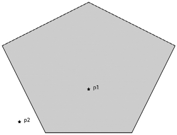
Figure 8.2 – Points inside and outside a polygonal region

Once we plot the points and the polygon it is easy (for us) to see that p1 lies inside the polygon and p2 does not. The contains method on the polygon object correctly classifies the points too.

How it works...

The Shapely Polygon class is a representation of a polygon that stores its vertices as points. The region enclosed by the outer boundary – the five straight lines between the stored vertices – is obvious to us and easily identified by the eye, but the notion of being inside the boundary is difficult to define in a way that can be easily understood by a computer. It is not even straightforward to give a formal mathematical definition of what it means to lie within a given curve.

There are two main ways to determine whether a point lies within a simple closed curve – that is, a curve that starts and ends at the same place that does not contain any self-intersections. The first uses a mathematical concept called the winding number, which counts the number of times the curve wraps around a point, and the ray crossing counting method, where we count the number of times a ray from the point to a point at infinity crosses the curve. Fortunately, we don’t need to compute these numbers ourselves since we can use the tools from the Shapely package to do this computation for us. This is what the contains method of a polygon does (under the hood, Shapely uses the GEOS library to perform this calculation).

The Shapely Polygon class can be used to compute many quantities associated with these planar figures, including perimeter length and area. The contains method is used to determine whether a point, or a collection of points, lies within the polygon represented by the object (there are some limitations regarding the kinds of polygons that can be represented by this class). In fact, you can use the same method to determine whether one polygon is contained within another since, as we have seen in this recipe, a polygon is represented by a simple collection of points.

Finding edges in an image

Finding edges in images is a good way of reducing a complex image that contains a lot of noise and distractions to a very simple image containing the most prominent outlines. This can be useful as our first step of the analysis process, such as in image classification, or as the process of importing line outlines into computer graphics software packages.

In this recipe, we will learn how to use the scikit-image package and the Canny algorithm to find the edges in a complex image.

Getting ready

For this recipe, we will need to import the Matplotlib pyplot module as plt, the imread routine from the skimage.io module, and the canny routine from the skimage.feature module:

import matplotlib.pyplot as plt
from skimage.io import imread
from skimage.feature import canny

The canny routine implements the edge detection algorithm. Let’s see how to use it.

How to do it…

Follow these steps to learn how to use the scikit-image package to find edges in an image:

1. Load the image data from the source file. This can be found in the GitHub repository for this chapter. Crucially, we pass in as_gray=True to load the image in grayscale:

   image = imread("mandelbrot."ng", as_gray=True)

The following is the original image, for reference. The set itself is shown by the white region and, as you can see, the boundary, indicated by the darker shades, is very complex:

Figure 8.3 – Plot of the Mandelbrot set generated using Python

2. Next, we use the canny routine, which needs to be imported from the features module of the scikit-image package. The sigma value is set to 0.5 for this image:

   edges = canny(image, sigma=0.5)
3. Finally, we add the edges image to a new figure with a grayscale (reversed) color map:

   fig, ax = plt.subplots()

   ax.imshow(edges, cmap="gray_r")

   ax.set_axis_off()

The edges that have been detected can be seen in the following image. The edge-finding algorithm has identified most of the visible details of the boundary of the Mandelbrot set, although it is not perfect (this is an estimate, after all):

Figure 8.4 – The edges of the Mandelbrot set found using the scikit-image package’s Canny edge detection algorithm

We can see that the edge detection has identified a good amount of the complexity of the edge of the Mandelbrot set. Of course, the boundary of the true Mandelbrot set is a fractal and has infinite complexity.

How it works...

The scikit-image package provides various utilities and types for manipulating and analyzing data derived from images. As the name suggests, the canny routine uses the Canny edge detection algorithm to find edges in an image. This algorithm uses the intensity gradients in the image to detect edges, where the gradient is larger. It also performs some filtering to reduce the noise in the edges it finds.

The sigma keyword value we provided is the standard deviation of the Gaussian smoothing that’s applied to the image prior to calculating the gradients for edge detection. This helps us remove some of the noise from the image. The value we set (0.5) is smaller than the default (1), but it does give us a better resolution in this case. A large value would obscure some of the finer details in the boundary of the Mandelbrot set.

Triangulating planar figures

As we saw in Chapter 3, Calculus and Differential Equations, we often need to break down a continuous region into smaller, simpler regions. In earlier recipes, we reduced an interval of real numbers into a collection of smaller intervals, each with a small length. This process is usually called discretization. In this chapter, we are working with two-dimensional figures, so we need a two-dimensional version of this process. For this, we’ll break a two-dimensional figure (in this recipe, a polygon) into a collection of smaller and simpler polygons. The simplest of all polygons are triangles, so this is a good place to start for two-dimensional discretization. The process of finding a collection of triangles that tiles a geometric figure is called triangulation.

In this recipe, we will learn how to triangulate a polygon (with a hole) using the Shapely package.

Getting ready

For this recipe, we will need the NumPy package imported as np, the Matplotlib package imported as mpl, and the pyplot module imported as plt:

import matplotlib as mpl
import matplotlib.pyplot as plt
import numpy as np

We also need the following items from the Shapely package:

from shapely.geometry import Polygon
from shapely.ops import triangulate

Let’s see how to use the triangulate routine to triangulate a polygon.

How to do it...

The following steps show you how to triangulate a polygon with a hole using the Shapely package:

1. First, we need to create a Polygon object that represents the figure that we wish to triangulate:

   polygon = Polygon(

       [(2.0, 1.0), (2.0, 1.5), (-4.0, 1.5), (-4.0, 0.5),

       (-3.0, -1.5), (0.0, -1.5), (1.0, -2.0), (1.0,-0.5),

       (0.0, -1.0), (-0.5, -1.0), (-0.5, 1.0)],

       holes=[np.array([[-1.5, -0.5], [-1.5, 0.5],

       [-2.5, 0.5], [-2.5, -0.5]])]

   )
2. Now, we should plot the figure so that we can understand the region that we will be working within:

   fig, ax = plt.subplots()

   plt_poly = mpl.patches.Polygon(polygon.exterior.coords,

       ec=(0,0,0,1), fc=(0.5,0.5,0.5,0.4), zorder=0)

   ax.add_patch(plt_poly)

   plt_hole = mpl.patches.Polygon(

       polygon.interiors[0].coords, ec="k", fc="w")

   ax.add_patch(plt_hole)

   ax.set(xlim=(-4.05, 2.05), ylim=(-2.05, 1.55))

   ax.set_axis_off()

This polygon can be seen in the following image. As we can see, the figure has a hole in it that must be carefully considered:

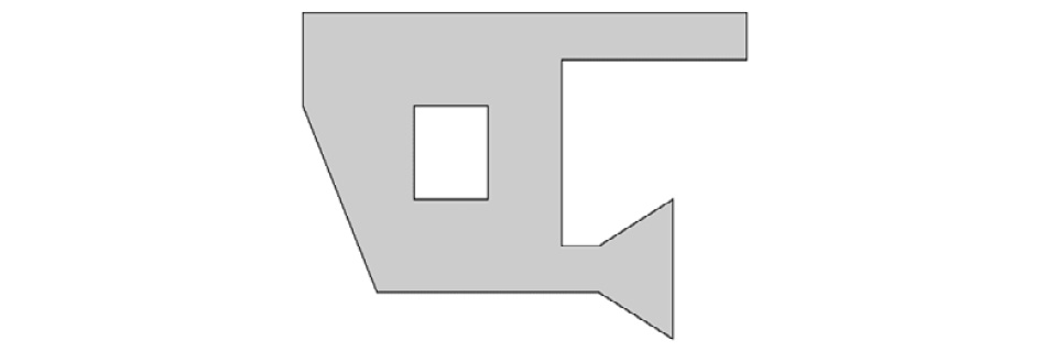
Figure 8.5 – Sample polygon but with a hole

3. We use the triangulate routine to generate a triangulation of the polygon. This triangulation includes external edges, which is something we don’t want in this recipe:

   triangles = triangulate(polygon)
4. To remove the triangles that lie outside the original polygon, we need to use the built-in filter routine, along with the contains method (seen earlier in this chapter):

   filtered = filter(lambda p: polygon.contains(p),

       triangles)
5. To plot the triangles on top of the original polygon, we need to convert the Shapely triangles into Matplotlib Patch objects, which we store in a PatchCollection:

   patches = map(lambda p: mpl.patches.Polygon(

       p.exterior.coords), filtered)

   col = mpl.collections.PatchCollection(

       patches, fc="none", ec="k")
6. Finally, we add the collection of triangular patches to the figure we created earlier:

   ax.add_collection(col)

The triangulation that’s been plotted on top of the original polygon can be seen in the following figure. Here, we can see that every vertex has been connected to two others to form a system of triangles that covers the entire original polygon:

Figure 8.6 – Triangulation of a sample polygon with a hole

The internal lines between the vertices of the original polygon in Figure 8.6 divide the polygon into 15 triangles.

How it works...

The triangulate routine uses a technique called Delaunay triangulation to connect a collection of points to a system of triangles. In this case, the collection of points is the vertices of the polygon. The Delaunay method finds these triangles in such a way that none of the points are contained within the circumcircle of any of the triangles. This is a technical condition of the method, but it means that the triangles are chosen efficiently, in the sense that it avoids very long, thin triangles. The resulting triangulation makes use of the edges that are present in the original polygon and also connects some of the external edges.

In order to remove the triangles that lie outside of the original polygon, we use the built-in filter routine, which creates a new iterable by removing the items that the criterion function falls under. This is used in conjunction with the contains method on Shapely Polygon objects to determine whether each triangle lies within the original figure. As we mentioned previously, we need to convert these Shapely items into Matplotlib patches before they can be added to the plot.

There’s more...

Triangulations are usually used to reduce a complex geometric figure into a collection of triangles, which are much simpler for computational tasks. However, they do have other uses. One particularly interesting application of triangulations is to solve the art gallery problem. This problem concerns finding the maximum number of guards that are necessary to guard an art gallery of a particular shape. Triangulations are an essential part of Fisk’s simple proof of the art gallery theorem, which was originally proved by Chvátal.

Suppose that the polygon from this recipe is the floor plan for an art gallery and that some guards need to be placed on the vertices. A small amount of work will show that you’ll need three guards to be placed at the polygon’s vertices for the whole museum to be covered. In the following image, we have plotted one possible arrangement:

Figure 8.7 – One possible solution to the art gallery problem where guards are placed on vertices

In Figure 8.7 here, the guards are indicated by the X symbols and their corresponding fields of vision are shaded. Here, you can see that the whole polygon is covered by at least one color. The solution to the art gallery problem – which is a variation of the original problem – tells us that we need, at most, four guards.

See also

More information about the art gallery problem can be found in the classic book by O’Rourke: O’Rourke, J. (1987). Art gallery theorems and algorithms. New York: Oxford University Press.

Computing convex hulls

A geometric figure is said to be convex if every pair of points within the figure can be joined using a straight line that is also contained within the figure. Simple examples of convex bodies include points, straight lines, squares, circles (disks), regular polygons, and so on. The geometric figure shown in Figure 8.5 is not convex since the points on the opposite sides of the hole cannot be connected by a straight line that remains inside the figure.

Convex figures are simple from a certain perspective, which means they are useful in a variety of applications. One problem involves finding the smallest convex set that contains a collection of points. This smallest convex set is called the convex hull of the set of points.

In this recipe, we’ll learn how to find the convex hull of a set of points using the Shapely package.

Getting ready

For this recipe, we will need the NumPy package imported as np, the Matplotlib package imported as mpl, and the pyplot module imported as plt:

import numpy as np
import matplotlib as mpl
import matplotlib.pyplot as plt

We will also need a default random number generator from NumPy. We can import this as follows:

from numpy.random import default_rng
rng = default_rng(12345)

Finally, we will need to import the MultiPoint class from Shapely:

from shapely.geometry import MultiPoint

How to do it...

Follow these steps to find the convex hull of a collection of randomly generated points:

1. First, we generate a two-dimensional array of random numbers:

   raw_points = rng.uniform(-1.0, 1.0, size=(50, 2))
2. Next, we create a new figure and plot these raw sample points on this figure:

   fig, ax = plt.subplots()

   ax.plot(raw_points[:, 0], raw_points[:, 1], "kx")

   ax.set_axis_off()

These randomly generated points can be seen in the following figure. The points are roughly spread over a square region:

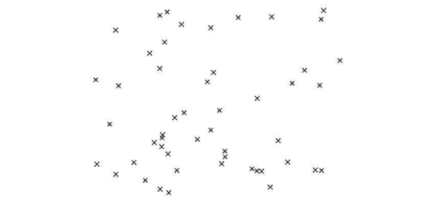
Figure 8.8 – A collection of points on the plane

3. Next, we construct a MultiPoint object that collects all these points and put them into a single object:

   points = MultiPoint(raw_points)
4. Now, we get the convex hull of this MultiPoint object using the convex_hull attribute:

   convex_hull = points.convex_hull
5. Then, we create a Matplotlib Polygon patch that can be plotted onto our figure to show the result of finding the convex hull:

   patch = mpl.patches.Polygon(

       convex_hull.exterior.coords,

       ec=(0,0,0,1), fc=(0.5,0.5,0.5,0.4), lw=1.2)
6. Finally, we add the Polygon patch to the figure to show the convex hull:

   ax.add_patch(patch)

The convex hull of the randomly generated points can be seen in the following figure:

Figure 8.9 – The convex hull of a collection of points on the plane

The polygon shown in Figure 8.9 has vertices selected from the original points and all the other points lie within the shaded region.

How it works...

The Shapely package is a Python wrapper around the GEOS library for geometric analysis. The convex_hull attribute of Shapely geometric objects calls the convex hull computation routine from the GEOS library, resulting in a new Shapely object. From this recipe, we can see that the convex hull of the collection of points is a polygon with vertices at the points that are farthest away from the center.

Constructing Bezier curves

Bezier curves, or B-splines, are a family of curves that are extremely useful in vector graphics – for instance, they are commonly used in high-quality font packages. This is because they are defined by a small number of points that can then be used to inexpensively calculate a large number of points along the curve. This allows detail to be scaled according to the needs of the user.

In this recipe, we’ll learn how to create a simple class representing a Bezier curve and compute a number of points along it.

Getting ready

In this recipe, we will use the NumPy package imported as np, the Matplotlib pyplot module imported as plt, and the comb routine from the Python Standard Library math module, imported under the binom alias:

from math import comb as binom
import matplotlib.pyplot as plt
import numpy as np

How to do it...

Follow these steps to define a class that represents a Bezier curve that can be used to compute points along the curve:

1. The first step is to set up the basic class. We need to provide the control points (nodes) and some associated numbers to instance attributes:

   class Bezier:

       def __init__(self, *points):

           self.points = points

           self.nodes = n = len(points) - 1

           self.degree = l = points[0].size
2. Still inside the __init__ method, we generate the coefficients for the Bezier curve and store them in a list on an instance attribute:

   self.coeffs = [binom(n, i)*p.reshape(

       (l, 1)) for i, p in enumerate(points)]
3. Next, we define a __call__ method to make the class callable. We load the number of nodes from the instance into a local variable for clarity:

       def __call__(self, t):

           n = self.nodes
4. Next, we reshape the input array so that it contains a single row:

           t = t.reshape((1, t.size))
5. Now, we generate a list of arrays of values using each of the coefficients in the coeffs attribute for the instance:

           vals = [c @ (t**i)*(1-t)**(n-i) for i,

              c in enumerate(self.coeffs)]

Finally, we sum all the arrays that were constructed in step 5 and return the resulting array:

       return np.sum(vals, axis=0)

6. Now, we will test our class using an example. We’ll define four control points for this example:

   p1 = np.array([0.0, 0.0])

   p2 = np.array([0.0, 1.0])

   p3 = np.array([1.0, 1.0])

   p4 = np.array([1.0, 3.0])
7. Next, we set up a new figure for plotting, and plot the control points with a dashed connecting line:

   fig, ax = plt.subplots()

   ax.plot([0.0, 0.0, 1.0, 1.0],

        [0.0, 1.0, 1.0, 3.0], "*--k")

   ax.set(xlabel="x", ylabel="y",

       title="Bezier curve with 4 nodes, degree 3")
8. Then, we create a new instance of our Bezier class using the four points we defined in step 7:

   b_curve = Bezier(p1, p2, p3, p4)
9. We can now create an array of equally spaced points between 0 and 1 using linspace and compute the points along the Bezier curve:

   t = np.linspace(0, 1)

   v = b_curve(t)
10. Finally, we plot this curve on top of the control points that we plotted earlier:

    ax.plot(v[0,:], v[1, :], "k")

The Bezier curve that we’ve plotted can be seen in the following diagram. As you can see, the curve starts at the first point (0, 0) and finishes at the final point (1, 3):

Figure 8.10 – Bezier curve of degree 3 constructed using four nodes

The Bezier curve in Figure 8.10 is tangent to the vertical lines at the endpoints and smoothly connects these points. Notice that we only have to store the four control points in order to reconstruct this curve with arbitrary accuracy; this makes Bezier curves very efficient to store.

How it works...

A Bezier curve is described by a sequence of control points, from which we construct the curve recursively. A Bezier curve with one point is a constant curve that stays at that point. A Bezier curve with two control points is a line segment between those two points:

When we add a third control point, we take the line segment between the corresponding points on the Bezier curve of curves that are constructed with one less point. This means that we construct the Bezier curve with three control points using the following formula:

This construction can be seen in the following diagram:

Figure 8.11 – Construction of a quadratic Bezier curve using a recursive definition (the two linear Bezier curves are shown by the dashed lines)

The construction continues in this manner to define the Bezier curve on any number of control points. Fortunately, we don’t need to work with this recursive definition in practice because we can flatten the formulae into a single formula for the curve, which is given by the following formula:

Here, the elements are the control points, is a parameter, and each term involves the binomial coefficient:

Remember that the parameter is the quantity that is changing to generate the points of the curve. We can isolate the terms in the previous sum that involve and those that do not. This defines the coefficients that we defined in step 2, each of which is given by the following code fragment:

binom(n, i)*p.reshape((l, 1))

We reshape each of the points, p, in this step to make sure it is arranged as a column vector. This means that each of the coefficients is a column vector (as a NumPy array) consisting of the control points scaled by the binomial coefficients.

Now, we need to specify how to evaluate the Bezier curve at various values of . This is where we make use of the high-performance array operations from the NumPy package. We reshaped our control points as column vectors when forming our coefficients. In step 4, we reshaped the input, , values to make a row vector. This means that we can use the matrix multiplication operator to multiply each coefficient by the corresponding (scalar) value, depending on the input, . This is what happens in step 5, inside the list comprehension. In the following line, we multiply the array by the array to obtain an array:

c @ (t**i)*(1-t)**(n-i)

We get one of these for each coefficient. We can then use the np.sum routine to sum each of these arrays to get the values along the Bezier curve. In the example provided in this recipe, the top row of the output array contains the values of the curve and the bottom row contains the values of the curve. We have to be careful when specifying the axis=0 keyword argument for the sum routine to make sure the sum takes over the list we created, and not the arrays that this list contains.

The class we defined is initialized using the control points for the Bezier curve, which are then used to generate the coefficients. The actual computation of the curve values is done using NumPy, so this implementation should have relatively good performance. Once a specific instance of this class has been created, it functions very much like a function, as you might expect. However, no type-checking is done here, so we can only call this function with a NumPy array as an argument.

There’s more...

Bezier curves are defined using an iterative construction, where the curve with points is defined using the straight line connecting the curves defined by the first and last points. Keeping track of the coefficient of each of the control points using this construction will quickly lead you to the equation we used to define the preceding curve. This construction also leads to interesting – and useful – geometric properties of Bezier curves.

As we mentioned in the introduction to this recipe, Bezier curves appear in many applications that involve vector graphics, such as fonts. They also appear in many common vector graphics software packages. In these software packages, it is common to see quadratic Bezier curves, which are defined by a collection of three points. However, you can also define a quadratic Bezier curve by supplying the two endpoints, along with the gradient lines, at those points. This is more common in graphics software packages. The resulting Bezier curve will leave each of the endpoints along the gradient lines and connect the curve smoothly between these points.

The implementation we constructed here will have relatively good performance for small applications but will not be sufficient for applications involving rendering curves with a large number of control points at a large number of values. For this, it is best to use a low-level package written in a compiled language. For example, the bezier Python package uses a compiled Fortran backend for its computations and provides a much richer interface than the class we defined here.

Bezier curves can, of course, be extended to higher dimensions in a natural way. The result is a Bezier surface, which makes them very useful general-purpose tools for high-quality, scalable graphics.

Further reading

• A description of some common algorithms from computation geometry can be found in the following book: Press, W.H., Teukolsky, S.A., Vetterling, W.T., and Flannery, B.P., 2007. Numerical recipes: the art of scientific computing. 3rd ed. Cambridge: Cambridge University Press.
• For a more detailed account of some problems and techniques from computational geometry, check out the following book: O’Rourke, J., 1994. Computational geometry in C. Cambridge: Cambridge University Press.