Chapter 6
Hybrid Excitation Synchronous Machines 1
6.1. Description
6.1.1. Definition
A hybrid excitation synchronous machine (HESM) is a machine associating the features of permanent magnet synchronous machines (PMSM) and coiled rotor synchronous machines (CRSM). It is a class of synchronous machine where the excitation flux is obtained by the contribution of two sources: one part of the excitation flux is created by permanent magnets; the other part by one or more excitation coils. This definition shows that the hybrid excitation concept is not linked to the synchronous machine. We could, for instance, design linear hybrid excitation actuators, or even hybrid excitation DC machines. We will exploit this to explain the simple functioning principle of hybrid excitation structures. The aim of such an association is obviously to associate the advantages of the two types of classical synchronous machines, i.e. a high mass and volume torque for PMSM and control of the excitation flux for CRSM.
In the first approach, excitation flux ![]() exc can be written as the sum of two fluxes: one generated by magnets
exc can be written as the sum of two fluxes: one generated by magnets ![]() a (which we will refer to as the magnet flux) and one generated by the excitation coils
a (which we will refer to as the magnet flux) and one generated by the excitation coils ![]() f (called the flux of excitation coils). This is summarized by the following equation:
f (called the flux of excitation coils). This is summarized by the following equation:
[6.1] ![]()
This approach assumes the linearity of the ferromagnetic materials used to build the machine. This type of formula allows us, to some extent, to take into account the magnetic saturation, as shown in Figure 6.1.
Figure 6.1. Evolution of excitation flux as a function of excitation current

This figure illustrates the evolution of maximum excitation flux as a function of excitation current typical of a HESM. The magnet flux is the excitation flux obtained for a zero excitation current. For a given current (for instance 3 A in Figure 6.1), the coil flux represents the difference between the total flux and the magnet flux.
The applications for which these machines can be competitive compared to existing machines are chiefly linked to transportation: electrical or hybrid vehicles and avionics. In the case of vehicles, these machines possess an additional degree of freedom (with respect to permanent magnet machines), which allows them to optimize the energy output on a running cycle [AMA 01]. In avionics, the HESM can be a good replacement for three-stage synchronous generators used to supply the onboard network, since they possess the same features (autonomous functioning and control of the excitation current to ensure a steady voltage) while having much less complex geometrical structures [PAT 06b]. From now on, we propose to classify HESMs.
6.1.2. Classification
Several classifications can discriminate between the various types of HESM (field lines, running as a motor or generator, structure). Here we use the most classic method, which separates the machines according to the field lines created by the two magnetic excitation sources [AMA 01, AMA 09, HLI 08, TAK 07]. We thus have two large classes of machines:
– HESM in series: the field lines generated by the excitation coils go through the magnets;
– HESM in parallel: the field lines generated by the excitation coils take a different path that allows the generation of flux without going through the magnets.
We will now present the features of machines falling into these two classes. We will associate one or more prototypes with each principle diagram.
6.1.2.1. HESMs in series
In this structure, the coil flux goes through the permanent magnets. This structure can be represented by a diagram of the basic electromagnetic actuator type (see Figure 6.2). The armature coil collects the excitation flux generated by the magnet and the excitation coil. The two excitation sources are assembled on the same branch of the magnetic circuit. Figure 6.3 shows a three-phase machine, with distributed winding and two pole pairs.
Figure 6.2. Principle diagram of a hybrid excitation structure in series

Figure 6.3. Principle diagram of a HESM in series

In these conditions, Figures 6.4 and 6.5 show that the excitation flux results from the contribution of flux generated by the permanent magnets and by the excitation coils. The flux of the excitation coil can be added to the magnet flux (overfluxing, see Figure 6.4) or be opposed to it (flux weakening, see Figure 6.5).
Figure 6.4. Overfluxing

Figure 6.5. Flux weakening
As indicated by the name of the structure, we notice that the field line generated by the excitation coil goes through the permanent magnet.
Figures 6.6 and 6.7 show the design of HESMs in series. In Figure 6.6, the machine has a distributed winding. The rotor (six pairs of poles) has smooth poles, the magnets are assembled at the surface and the excitation coils are localized on the rotor. We can see this structure as a CRSM possessing an air-gap that is sufficiently large for magnets be put therein.
Figure 6.6. A HESM in series [AMA 09]

Figure 6.7 shows a prototype of a HESM with flux commutation (passive rotor). The excitation sources are in the stator, thus allowing us to discard the rings and sliding contacts.
The major advantage of HESMs in series lies in them running in flux weakening. The generation of a coil flux opposed to the magnet flux occurring at every point of the machine, the decrease in flux will lead to a decrease in iron losses (with Joule losses, however, due to the excitation coil). Hence, to some extent it will lead to an improvement in output in flux weakening zones.
Figure 6.7. A HESM in series [AMA 09]

The major drawback of these structures is linked to their principle: the efficiency of the excitation coils is reduced by traveling through the magnet, the magnet being considered comparable with an important air-gap. In flux weakening mode there is a risk of demagnetization of the magnet by the excitation coils. It is necessary to take this into account during the dimensioning step of this type of machine. This problem makes it impossible to completely cancel the excitation flux.
The HESMs in parallel, which we present hereafter, allow us to partially solve this problem.
6.1.2.2. HESMs in parallel
When the flux of the excitation coils does not travel through the magnets, the HESMs are referred to as being in parallel. In this case, the HESMs’ topologies can be reduced in number by the inventiveness of machine designers. Here, we restrict ourselves to presenting the functioning principle of these structures. For a more exhaustive analysis, we invite the reader to refer to [AMA 01, AMA 09] and [HLI 08]. From a global point of view, all these structures can be classified in two subcategories: HESMs in parallel, with or without short-circuit. We will describe these in the following sections.
6.1.2.2.1. HESMs in parallel with short circuit
When the excitation current is 0, the excitation flux is also 01 . For the magnet flux, there is a less reluctant path than that through the armature coil, as illustrated in Figure 6.8. In the absence of excitation current, the magnet flux is entirely picked up (short circuit, see Figure 6.7) by the excitation coil, and the flux collected by the armature coil is 0. HESMs using this principle therefore work rather like CRSMs whose excitation fluxes are improved thanks to the presence of permanent magnets.
Figure 6.8. Principle diagram of a hybrid excitation structure in parallel

Figure 6.9 shows the principle of a rotating machine that works according to this principle.
Figure 6.9. Principle diagram of a HESM in parallel

The functioning principle of these HESMs is shown in parallel in Figure 6.10 and with a short circuit in Figure 6.11.
Figure 6.10. Short-circuit of the magnet flux

When the excitation coil is supplied, the magnet flux is progressively orientated towards the armature coil due to saturation of the magnetic branch having the excitation coil (see Figure 6.11). There does remain, however, the presence of a loss of flux.
Figure 6.11 is dedicated to the explanation of the overfluxing mode.
Figure 6.11. Overfluxing

Figure 6.12 presents the rotor of a real machine using this process (the stator is a classic stator with distributed winding). It is the claw-pole (or Lundell) machine, to which we have added magnets between the claws, referred to as inter-claw magnets. The excitation coil is global (not visible in Figure 6.12 because it is located under the claws).
The aim of these structures in parallel with short-circuit is to run safely. They allow us to fix a problem met by PMSMs supplied by an inverter during a defect in a short circuit on one of the bridge arms. In this case, the short-circuit current is only limited by the stator resistance and stator cyclical inductance of the PMSMs. With these HESMs in parallel and with short circuit, we can cancel out the excitation current in order to cancel out the short-circuit current. Safety is ensured even if the circuit supplying the coiled inductor shows a defect. Furthermore, if the magnet represents an important air-gap before the stator-rotor air-gap, the risk of demagnetizing the magnet due to the coiled excitation is considerably decreased.
Figure 6.12. Rotor of the hybrid excitation claw-pole machine [TAK 07]

A few drawbacks of such structures need to be pointed out here:
– no matter what the function contemplated (overfluxing or flux weakening), part of the magnet flux is irremediably lost (see the losses flux in Figure 6.7);
– if HESMs are in series, the excitation coils do not work optimally;
– in HESMs in parallel, the magnet is not used completely;
– running is possible at the expense of Joule losses at the excitation circuit level.
HESMs without short circuit allows us to solve this problem to some extent. They are the topic of the following section.
6.1.2.2.2. HESM in parallel without short circuit
HESMs in parallel and without short circuit allow us to obtain a non-zero excitation flux, even if the excitation current is 0. Figure 6.13 shows an actuator that illustrates this principle. We will notice that a leakage flux exists that is characteristic of HESMs in parallel.
Figure 6.13. Principle diagram of a hybrid excitation structure in parallel

In this figure, we can notice that the excitation coils are represented in the stator. Figure 6.14 shows a rotating structure using the same principle.
Figure 6.14. Principle diagram of a HESM in parallel

Figures 6.15 and 6.16 show the effect of excitation coils.
Figure 6.15. Overfluxing

During the operation in flux weakening mode, however, there are zones where the global flux increases. In this type of structure, flux weakening does not necessarily lead to a decrease in iron losses.
Figure 6.16. Flux weakening

Figures 6.17 and 6.18 show HESMs in parallel without short circuits. In the first structure (see Figure 6.17), the principle consists of taking a permanent magnet machine with flux concentration and replacing every other magnet with an excitation coil.
Figure 6.17. HESM in parallel [AMA 09]

This type of construction is applicable to practically every permanent magnet machine. Finally, Figure 6.18 shows a machine with hybrid excitation and flux commutation.
Figure 6.18. HESM with hybrid excitation andflux commutation [HOA 07]

Generally, running safety is ensured by these structures while the supply circuit of the inductor does not show defects at the same time as the armature. The excitation flux exists even in the absence of an excitation current, so these HESMs are good candidates for applications requiring the minimization of losses on a running cycle [AMA 01]. With these machines in series, the efficiency of the excitation coil is much better, since the coils do not have to overcome the reluctance produced by the permanent magnet.
6.2. Modeling with the aim of control
6.2.1. Setting up equations
Modeling the HESM involves the same principles as the classic synchronous machines. Assuming that the action of magnets is identical to that of the excitation coil, we can write the vector of stator fluxes as follows:
with:

where p is the number of pole pairs of the machine, ![]() is the angular position of the rotor with respect to the stator (see Figure 6.19 describing the equivalent bipolar machine thus modeled) and kH is a hybridization coefficient characterizing the contribution of the excitation current in the global excitation flux. We will note that for the boundary cases:
is the angular position of the rotor with respect to the stator (see Figure 6.19 describing the equivalent bipolar machine thus modeled) and kH is a hybridization coefficient characterizing the contribution of the excitation current in the global excitation flux. We will note that for the boundary cases:
– kH = 0 corresponds to a machine with permanent magnets only;
– kH![]() 1 corresponds to a machine with coiled excitation alone.
1 corresponds to a machine with coiled excitation alone.
Figure 6.19. Equivalent bipolar HESM

In this model, we will consider a synchronous machine that potentially has salient poles, i.e. with a matrix of stator inductances (Lss) function of the angular position of the rotor with respect to the stator. The classical formulation of the first harmonics of this matrix, written (Lss(![]() )) is:
)) is:
with:

and:

The classical factorizations of these matrices call for Concordia matrices T32 and rotation matrices P(.), defined as follows:

We notice then that:
and matrix (Lss2(![]() )) can be written in the following way:
)) can be written in the following way:
where matrix K2 is a 2 × 2 matrix similar to the conjugation operation for complex numbers. It is written as:
![]()
The vectorial equation of stator fluxes must be completed by that of the flux generated in the excitation coil, i.e.
In this equation, we have the reciprocity of the action between the stator armature coils and excitation coil. We also notice that the flux generated by the magnet in this excitation coil can be different from that generated in the armature coils by introducing a new parameter ![]() ′0 that, as we can see, has no influence on the voltage equations of the machine, since it is a constant. In fact, the voltage equations, both for the armature and the excitation coil, are obtained by application of Faraday’s and Ohm’s laws at the level of the coil:
′0 that, as we can see, has no influence on the voltage equations of the machine, since it is a constant. In fact, the voltage equations, both for the armature and the excitation coil, are obtained by application of Faraday’s and Ohm’s laws at the level of the coil:
and
[6.9] ![]()
As a consequence, the application of dq transformation (i.e. ![]()
![]() transformation plus rotation in the rotor reference frame with the excitation flux axis being d) leads us to the following dq equations (in reference frame dq):
transformation plus rotation in the rotor reference frame with the excitation flux axis being d) leads us to the following dq equations (in reference frame dq):
where J2 is the matricial analogue of the pure imaginary j for complex numbers (i.e. j2= -1):
![]()
and the armature flux equation gives:
where I2 is the second-order identity matrix.
Similarly, we can re-write:
[6.12] ![]()
Representation in the form of electrical diagrams is a natural goal for the electrical engineer and it is therefore interesting to address this formulation problem in the case of HESMs. The classical minimum solution is to describe the three-phase armature coils using a unique “single-phase” diagram. In the case of a dynamic model (that can be used to describe transient regimes), this single-phase representation requires the use of phasors that can be directly introduced from a real dq modeling. For this purpose, we can introduce the definition of a phasor xs = xd + jxq.
We then obtain the phasor equation of the stator armature voltages:
with:
The major problem with this phasor modeling comes from the presence of a conjugation operation in the stator flux equation. This conjugation comes from the saliency term of the machine’s inductance (Lss(![]() )). It is therefore impossible to propose an equivalent electrical diagram without introducing a new component in the classic electrical library (consisting of voltage sources, resistances, capacitors, inductances and ideal transformers). Hence, it is preferable to give up a unified representation of equations on the two axes (d and q) of the machine in order to look for a representation using components. Physically, this is justified by the anisotropy of the salient pole machines, contrary to machines with smooth poles, such as asynchronous machines that allow a simple phasor representation.
)). It is therefore impossible to propose an equivalent electrical diagram without introducing a new component in the classic electrical library (consisting of voltage sources, resistances, capacitors, inductances and ideal transformers). Hence, it is preferable to give up a unified representation of equations on the two axes (d and q) of the machine in order to look for a representation using components. Physically, this is justified by the anisotropy of the salient pole machines, contrary to machines with smooth poles, such as asynchronous machines that allow a simple phasor representation.
REMARK 6.1. in the case of the synchronous machine with smooth poles, we again find the isotropic behavior of the machine so it is therefore possible to find the phasor representation but there is always an error source − the “purely real” excitation in this complex representation. This error in some way generates anisotropy by favoring axis d. This is all the more true in the case of a magnetically-saturated machine.
6.2.2. Formulation in components
To write equations in components of HESMs, we are going to introduce the following parameters:
– armature inductance of axis d: Ld = Ls0 − Ms0 + Ls2;
– armature inductance of axis q: Lq = Ls0 − Ms0 − Ls2;
– magnetic flux (constant) in ![]()
![]() reference frame:
reference frame: ![]() ; and
; and
– mutual inductance between the armature and excitation coil: M = kH.![]() 0.
0.
The armature voltage equations (scalar) are then written:
with:
where from:
[6.20] ![]()
we see that two back-electromotive forces (back-emfs) appear in the two equations, which we will refer to as ed and eq, respectively, and whose expressions are:
These two back-emfs are representative of the electromechanical energy conversion in the machine and as a consequence we have the expression of instantaneous mechanical power, pm:
where cm is the instantaneous torque delivered by the HESM to the drive shaft (study in motor convention).
We then infer the electromechanical model of the machine with the expression of its torque as a function of electrical currents in the different coils:
[6.24] ![]()
Similarly to the introduction of ![]() exc(if,
exc(if, ![]() ) in the initial model (a,b,c) of the machine, in dq reference frame we can note an excitation flux
) in the initial model (a,b,c) of the machine, in dq reference frame we can note an excitation flux ![]() exc(if) in the form:
exc(if) in the form:
There is a last step left for handling the equations for the electrical model of the machine. It requires the choice of localization of the magnetizing inductance that accounts for the machine’s flux. We are going to proceed to modeling this in the form of a dynamic diagram in components (DDCs) of the HESMs by localizing the inductance at the level of the armature (on the equivalent circuit of axis d). In this case, we again take the equation of voltage, ![]() d, factorizing all the dynamic terms (i.e. in d/dt) by Ld:
d, factorizing all the dynamic terms (i.e. in d/dt) by Ld:
We then make a transformation ratio m appear, accounting for coupling between the component of axis d of the armature and the excitation coil: m = M/Ld. We have then emphasized a magnetizing current ![]() of the machine that accounts for its magnetic state:
of the machine that accounts for its magnetic state:
From these results we establish the equivalent diagram corresponding to axis d of the armature (see Figure 6.20). The diagram showing axis q of the armature, which completes the representation of the machine (see Figure 6.21), is immediately inferred from equation [6.20].
As indicated in the caption of Figure 6.20, this diagram is incomplete and more so for axis d because we see that current m.if is injected in the circuit without being linked to a described supply. It now remains for us to describe the excitation coil that will have to be “naturally” connected to the diagram of axis d of the armature in the form of an equivalent diagram. For this purpose, we again take equation [6.9] by using expression [6.12] of the flux in the excitation coil. We thus get:
[6.28] ![]()
Figure 6.20. Partial dynamic diagrams in components of the armature of the HESM (bottom) for axis d and (top) for axis q

For a connection to be possible between the diagram shown in Figure 6.20 and the circuit representing the excitation, hawse have to introduce voltage ![]() into this equation because we see current m.if appear in the armature circuit. We can then write:
into this equation because we see current m.if appear in the armature circuit. We can then write:
[6.29] ![]()
From equations [6.28] and [6.29], we can then write that:
[6.30] ![]()
In this equation, we make a dispersion coefficient ![]() appear that is expressed as:
appear that is expressed as:
The latter is similar to that existing in the asynchronous machine. It accounts for an imperfect coupling between axis d of the armature and the excitation coil. We will note that here the leakages have been added up at the level of the excitation coil.
This choice is arbitrary and we could have proceeded in the opposite way, with a magnetizing inductance placed at the level of the excitation coil and localizing the magnetic leakages on axis d of the armature. On the basis of equation [6.30] and of the partial diagrams in Figure 6.20, it is now possible to establish the complete DDCs of the HESMs, as indicated in Figure 6.21.
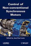
Figure 6.21. Complete dynamic diagram in components of the HESM

6.2.3. Complete model
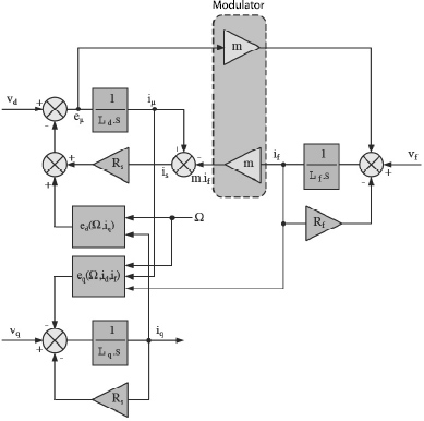
The complete model of the machine associates the components of the dynamic model with the electromechanical conversion and the mechanical load of the motor. This set is represented diagrammatically in Figure 6.22.
Figure 6.22. Complete model of HESM (electrical/electromechanical) and its mechanical load (here an inertial load with viscous friction and an additional resistant torque cr that is not defined)

The model above is directly implantable in a “functional” simulator, such as Matlab/Simulink, due to its block diagram-type structure. However, the DDCs in Figure 6.21 are not directly useable, so it is necessary to convert the figure to block diagrams. This operation can be done systematically for any electrical diagram [PAT 06] starting from state variables carried by reactive components (inductances and capacitors). Here, we have three state variables, which are:
– current in the excitation coil (if);
– magnetizing current ![]() ; and
; and
– the armature current of axis q, (iq).
The interconnections between the three associated integrators are obtained by the application of Kirschhoff’s laws and it eventually leads to the diagram in Figure 6.23.
Figure 6.23. Block diagrams corresponding to the DDCs in Figure 6.21 of an HESM
6.3. Control by model inversion
6.3.1. Aims of the torque control
The torque control of HESM requires the optimization of the three currents injected in the equivalent coils of the dq model of the machine. In fact, the torque generated by the machine is a function of these three currents, as shown by equation [6.24]. There is thus an important redundancy in the degrees of freedom available for piloting. In the case of a machine with smooth poles, the search for a maximum torque output for a minimum injected torque requires cancellation of the current of axis d to the advantage of the sole current, iq. Current id is eventually only used to overcome the limitations of the supply at high speed in order to ensure flux weakening of the machine.
This solution is no longer as easy in the case of machines with salient poles with the possibility of generating a torque of variable reluctance with the association of currents id and iq when Ld − Lq is not zero. The “balance” between these two components is a matter of a compromise between the benefit in torque brought by each component and the losses occurring in the machine. It is therefore an optimization problem of losses under torque constraint and possibly limitation of the voltage that can be provided by the uninterruptible power supply with a given DC bus voltage.
Finally, the situation is even more complicated with an HESM insofar as the magnetic flux of the machine is the superposition (in linear regime) of three sources:
– the permanent magnets;
– excitation current if; and
– armature current of axis d.
However, the process remains identical to that of machines with salient poles: it is about optimizing a criterion by gauging the contribution of each of these degrees of freedom.
As a consequence, we can see the torque control of HESMs as a structure organized into a hierarchy, such as that in Figure 6.6, in which the three input currents id, iq and if (applied at the inputs of three dedicated regulation loops) are controlled by an optimizer, where one of the constraints is the desired motor torque on the drive shaft of the machine. This input is hence a torque input that can itself come from the speed or position regulation loop of the machine according to the targeted application.
Figure 6.24. Block-diagrams corresponding to the DDCs in Figure 6.3 of the HESM
6.3.2. Current control of the machine
The torque piloting of HESMs physically requires current control in the coils of the machine. The regulation of these currents allows us to introduce limitations that have a safety role. Here, making a regulation loop can be based on an inversion control principle, in which control can be seen as the symmetrical process of the process thus piloted. We can illustrate this with the supply of the armature coil of axis q.
Figure 6.25. DDCs of axis q of the armature and its control

Figure 6.25 we see that the control must apply a voltage ![]() q equal to the sum of three voltages, Rs.iq, eq and Lq.diq/dt. The first two voltages can be compensated for in open loop because it is about rigid relationships (in the sense of causality); whereas the third is piloted by a corrector acting as a regulator in the closed loop of current iq. The control structure obtained is then that given in Figure 6.26.
q equal to the sum of three voltages, Rs.iq, eq and Lq.diq/dt. The first two voltages can be compensated for in open loop because it is about rigid relationships (in the sense of causality); whereas the third is piloted by a corrector acting as a regulator in the closed loop of current iq. The control structure obtained is then that given in Figure 6.26.
Figure 6.26. Regulation loop of current iq
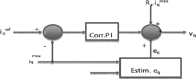
REMARK 6.2. we notice that to compensate for voltage drop at the terminals of Rs, we use the measure (written with the exponent “mea”) of current iq here. A second possibility consists of using the input and not the measure. In practice, this type of solution prevents us from adding a measuring noise in the control and bears the loss of the sensor because it is about control that is partially in open loop.
By proceeding similarly, we can establish the regulation loops for id and if in Figure 6.27.
For the regulation of id, we notice that it is about the regulation of ![]() , which is hidden from the point of view of input by piloting of the input
, which is hidden from the point of view of input by piloting of the input ![]() with the help of inputs id and if (i.e.
with the help of inputs id and if (i.e. ![]() and
and ![]() ).
).
When the three regulation loops are implanted, we can see the machine and its close control as a system relating to three reference inputs ![]() ,
, ![]() and
and ![]() , and a motor torque cm with controlled dynamics. In fact, the PI correctors used for each loop allow us to master the time constant of the system in closed loop (by pole placement) and the integrating effect of the corrector allows us to compensate for possible errors made in the compensation terms. The compensation terms are injected in the open loop in voltage inputs
, and a motor torque cm with controlled dynamics. In fact, the PI correctors used for each loop allow us to master the time constant of the system in closed loop (by pole placement) and the integrating effect of the corrector allows us to compensate for possible errors made in the compensation terms. The compensation terms are injected in the open loop in voltage inputs ![]() d,
d, ![]() q and
q and ![]() f applied to electronic power converters supplying the coils of the machine (inverter for the armature and chopper for the excitation).
f applied to electronic power converters supplying the coils of the machine (inverter for the armature and chopper for the excitation).
Figure 6.27. Regulation loops of id and if

6.3.3. Optimization and current inputs
As has already been mentioned, the three input currents are calculated by an optimizer in charge of obtaining the desired torque while minimizing a certain criterion: generally we try to minimize the losses in the machine (even in the converters). The function to be optimized is relatively complex and it is usually preferable to carry out the optimization work offline and to tabulate the inputs as a function of the different parameters, such as torque input and rotational speed of the machine.
The function to be optimized is relatively difficult to define, according to the model of losses used to describe the machine. In fact, we can include the iron losses and the mechanical losses, but here we are going to restrict ourselves to losses directly inferred from the model that was previously developed, i.e. copper losses pcu in the different coils:
Now criterion J(.), which is the easiest to optimize within this framework, consists of the addition of pcu, a constraint of the “equality on torque” type to this function by means of a Lagrange multiplier λ1:
Figure 6.28. Optimal currents to be injected in the machine as a function of the input torque (between -20 and +20 N.m) and the current rotational speed of the machine (between 0 and 4,000 rpm)

We can easily integrate an additional constraint on vectorial the emf (ed, eq) of the machine so that it remains smaller or equal to a certain value, Esmax, set by the uninterruptible power supply (for instance 90% of the maximum value of voltage vector (![]() d,
d, ![]() q)t that it can generate for DC bus voltage U0). In this boundary case, the optimization criterion is modified by the addition of a new Lagrange multiplier, λ2:
q)t that it can generate for DC bus voltage U0). In this boundary case, the optimization criterion is modified by the addition of a new Lagrange multiplier, λ2:
– equality between estimated torque cm(id,iq,if) and reference ![]() (associated with λ1);
(associated with λ1);
– equality between the back-emf of the armature and the maximum value allowed by the inverter, Esmax (associated with λ2).
We will notice that this control is not optimal in the classical sense (i.e. of automatics) but rather a suboptimal control, because it is only truly optimal in steady state (constant torque/speed). In practice, it has a high performance as long as the dynamics of the input torque remain slow with respect to the response times of the current regulation loops. This is most often verified in the targeted applications (e.g. electrical or hybrid vehicles).
6.4. Overspeed and flux weakening of synchronous machines
6.4.1. Generalities
The torque control presented in the previous section minimized losses in the machine for a given torque input (the first constraint to fulfill) while limiting the back-emf of the machine. This last constraint (inequality) is that consisting of decreasing the global flux undergone by the armature (if necessary). We will notice that the armature is the site of a back-emf proportional to the flux and to the rotational speed of the machine. This is similar to the scalar case of the DC machine (DCM) for which back-emf, E, in the armature is ruled by the relationship:
As a consequence, for a given supply (with a chopper, the supplied voltage lies between 0 and Udc), the speed can not exceed a value ![]() max so that:
max so that:
by assuming that the voltage drops in the armature (only in resistance in a DCM) are negligible.
In the case of a machine with adjustable excitation, we can control the value of ![]() as a function of an excitation current, if. In the case of a machine with linear functioning, we have a proportionality coefficient between these two variables,
as a function of an excitation current, if. In the case of a machine with linear functioning, we have a proportionality coefficient between these two variables, ![]() = Maf.if. We notice that when we want to increase the speed of the machine, we can decrease if because we then decrease k.
= Maf.if. We notice that when we want to increase the speed of the machine, we can decrease if because we then decrease k.![]() . Even in the case of a saturated machine, we have a monotonously increasing relationship between flux
. Even in the case of a saturated machine, we have a monotonously increasing relationship between flux ![]() and current if (which, at small if values, is almost linear), which leads to the same result.
and current if (which, at small if values, is almost linear), which leads to the same result.
6.4.2. Flux weakening of synchronous machines with classical magnets
This flux weakening function can be illustrated by a Behn-Eschenburg diagram for synchronous machines with smooth poles. In fact, for a given point of operation of the machine (in the torque-speed plane), we can define the single-phase vectorial diagram linking simple voltage and phase current by knowing the synchronous reactance Xs and by considering the negligible resistance Rs of the coil (see Figure 6.29). We will notice the voltage limit imposed by the inverter (amounting to 0.637 Udc in the case of a space-vector modulation in linear regime – i.e. without overmodulation) in the two diagrams proposed. In Figure 6.29a we notice that the inverter can supply the required voltage, V, while in Figure 6.29b it is impossible. The solution is given in Figure 6.29c, where we see that the addition of a current component Id < 0 on axis d decreases the amplitude of voltage vector V, which must be supplied by the inverter, and that the inverter enters the accessible zone. Obviously, the addition of component Id decreases the value of Iq available because we can also define a limit common to the inverter and the machine, which is admissible current by phase Imax and leads us to write the following inequality:
Figure 6.29. Behn-Eshenburg diagrams

6.4.3. The unified approach to flux weakening using “optimal inputs”
In the case of HESMs, we have seen that a current if was dedicated to the generation of the armature flux similarly to the magnets. It is also obvious in the DDCs established in Figure 6.21 that current if is not the only one to generate the armature flux. In fact, it is coupled with the armature current of axis d, written id. Now, current id is the only degree of freedom available for a possible flux weakening in synchronous machines with classical magnets. We can therefore distinguish two cases:
– The case of synchronous machines with smooth poles for which current id is only useful for the flux weakening insofar as it only intervenes in the expression of the motor torque.
– The case of machines with salient poles for which current id has an impact on the torque and the flux weakening of the machine.
The control technique previously proposed, however, tends to unify the optimal controls of the machine in the operating zones with constant available torque and power (i.e. flux weakening zone). It does this by the “tabulation” of input currents as a function of the operating point in the “torque/speed” plane.
REMARK 6.3.– This control principle is applicable not only to piloting of the machine by an inverter connected to a constant voltage source, but also in the case where the machine running as a generator, we wish to pilot voltage Udc. In this case, the three-phase transistor bridge behaves as a PWM rectifier [PAT 06a].
6.4. Conclusion
To conclude, we suggest a basic comparison between the structures of HESM presented. This comparison is summarized in Figure 6.30, which shows the evolution of the image of the excitation flux as a function of the excitation current. The results come from finite element calculations carried out from Figures 6.3, 6.9 and 6.14. The CRSM curve represents the results obtained from Figure 6.9, where the magnets have been replaced with air. It allows us to measure the contribution of permanent magnets (HESM in parallel with short circuit). The structures in series are those that feature the best configuration for permanent magnets (HESM S). In fact, they thus feature the highest excitation flux when the excitation current is 0. On the other hand, because of the reluctance shown by the magnet, the impact of excitation coils is strongly reduced. The efficiency2 of the hybrid excitation is therefore less important than for structures in parallel. The HESMs in parallel with short circuit feature 0 excitation flux for a flux of 0. For the HESM in parallel without short circuit, the excitation flux can be cancelled out at the expense of Joule excitation losses. This type of machine requires a bidirectional supply circuit in current, similar to machines in series. The modeling of the machines in this chapter aims to translate the behavior of the machine in the form of a valid electrical diagram, both in transient regime and in sinusoidal steady-state regime. It allows us, moreover, to emphasize the “good state variables” of the system to then lead to their piloting by inversion of the model. Finally, because of the redundancy of degrees of freedom in controlling the machine, we can determine optimal inputs on the basis of the model developed. These inputs can then be generated on the basis of a measure of rotational speed by a “supervisor” delivering the torque input required by the application. This approach is all the more interesting from the point of view of its implantation. It allows us to generate unified control of the machine on the torque/speed plane (within the physical limits allowed). In other words, thanks to an adapted optimization criterion it allows us to ensure the machine runs in the operating zone with constant available torque and in the zone limited by constant power (flux-weakening zone).
Figure 6.30. Basic comparison of the different classes of HESM (Key: CRSM = coiled rotor synchronous machines; PNSC = in parallel without short circuit; PSC = in parallel with short circuit; S = ?

6.5. Bibliography
[AMA 01] AMARA Y., Contribution à la commande et à la conception de machines synchrones à double excitation, PhD thesis, University of Paris XI, December 2001.
[AMA 09] AMARA Y., VIDO L., GABSI M., HOANG E., BEN AHMED A. H., LÉCRIVAIN M., “Hybrid excitation synchronous machines: Energy efficient solution for vehicle propulsion”, IEEE Transactions on Vehicular Technology, vol. 58, no. 5, pp. 2137-2149, 2009.
[HLI 08] HLIOUI S., Étude d’une machine synchrone à double excitation. Contribution à la mise en place d’une plate-forme de logiciels en vue d'un dimensionnement optimal, PhD thesis, UTBM, December 2008.
[HOA 07] HOANG E., LECRIVAIN M., GABSI M., “A new structure of a switching flux synchronous polyphased machine with hybrid excitation”, European Conference on Power Electronics and Applications, pp. 1-8, September 2007.
[PAT 06a] PATIN N., VIDO L., MONMASSON E., LOUIS J.-P., “Control of a DC generator based on a Hybrid Excitation Synchronous Machine connected to a PWM rectifier”, Proc. IEEE ISIE’06, CD ROM, Montreal, Canada, July 2006.
[PAT 06b] PATIN N., Analyse d’architectures, modélisation et commande de réseaux autonomes, PhD thesis, ENS Cachan, December 2006.
[TAK 07] TAKORABET A., Dimensionnement d’une machine à double excitation de structure innovante pour une application alternateur automobile. Comparaison à des structures classiques, PhD thesis, ENS Cachan, January 2007.
1 Chapter written by Nicolas PATIN and Lionel VIDO.
1 The model proposed by equation [6.1] does not allow us to describe this class of machine.
2 One calls efficiency of the double excitation the derivative of the excitation flux with respect to the excitation current.