MATLAB® basics
MATLAB® came into being in the 1970s as a tool for mathematicians and educators, but was soon adopted by engineers as an effective means for technical computing. Its name is a composite of the words ‘Matrix’ and ‘Laboratory’, emphasizing that its main element is the matrix. Such an approach permitted unification of the processes of various calculations, graphics, modeling, simulation and algorithm development. This chapter introduces the main windows and starting procedure, describes the main commands for simple arithmetic, algebraic and matrix operations, and presents the basic loops and relational and logical operators.
2.1 Starting with MATLAB®
MATLAB® can be installed on computers running different operation systems, but I will assume here that the reader uses a personal computer running a Windows operating system. To start one has simply to click on the MATLAB® icon (Figure 2.1) provided with a MATLAB® subscription; the icon is placed on the Quick Lunch bar or on the Windows Desktop. Another way to start the program is to select MATLAB® 20010a in the MATLAB®- directory in the ‘All Programs’ option of the Windows ‘Start’ menu.

Figure 2.1 MATLAB® icon (enlarged). The image can be produced with the logo command; the background color has been changed.
2.1.1 MATLAB® Desktop and its windows
The window that first opens is the MATLAB® Desktop (Figure 2.2), which comprises four windows: Command, Current Folder, Workspace and Command History.
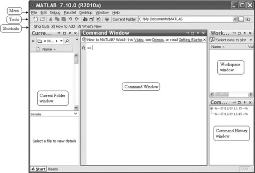
These are the most intensively used windows and are briefly described further. There are also Help, Editor and Figure windows that do not appear with the MATLAB® Desktop and are described in the chapters where they are used.
The Desktop also contains: the Menu, which can be changed depending on the tool being used; the MATLAB® Tools bar, which contains the more common functions; the Shortcuts bar, where one can place icons for quick running of MATLAB® programs or group commands; and the Start button, used to access various tools, demos, shortcuts and documentation.
The Command Window is the main outlet where commands are entered and results are displayed. Sometimes it is convenient to separate it from the desktop by clicking ![]() to the right of the title bar. Such separation is possible for all Desktop windows. To combine windows one has to click on
to the right of the title bar. Such separation is possible for all Desktop windows. To combine windows one has to click on ![]() or select the Default line in the Desktop Layout of the Desktop option at the Menu bar.
or select the Default line in the Desktop Layout of the Desktop option at the Menu bar.
Workspace is the graphical interface that allows us to view and manage the variables and other objects of the MATLAB® workspace; it also displays and automatically updates the values of each variable.
Current Folder presents a browser that shows the full path to the current folder, and shows the contents of the current folder. When starting MATLAB®, we view a starting directory which is called the startup directory. After selecting the file, information about it appears in the Details panel.
Command History stores the commands most recently entered in the Command Window.
2.1.2 Elementary functions and interactive calculations
Two main working modes are available in MATLAB® – interactive and with m-files. I will explain the latter in later chapters. The interactive mode is discussed briefly here.
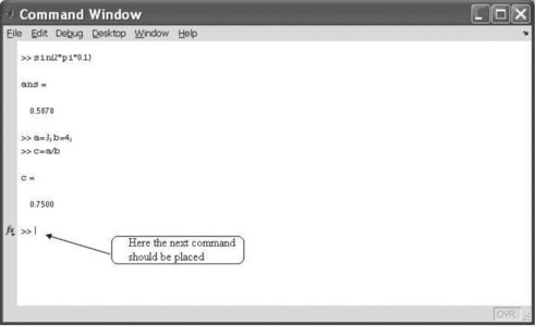
To enter and execute a command, it must be typed in the Command Window immediately after the command prompt >>. Figure 2.3 shows this window with some elementary commands.
The symbol ![]() , which appears in the most recent versions of MATLAB®, is called the Function Browser, and helps to find the function required and information about its syntax and usage.
, which appears in the most recent versions of MATLAB®, is called the Function Browser, and helps to find the function required and information about its syntax and usage.
Entering a command and manipulating with it require us to master the following operations:
• the command must be typed next to the prompt >>;
• the Enter key must be pressed for execution;
• a command in a preceding line cannot be changed; to correct or repeat an executed command the up-arrow key ↑ should be pressed;
• a long command can be continued in the next line by typing … – three periods; commands in the same line should be divided by semicolons (;) or by commas (,); a semicolon at the end of a command prevents the answer from being displayed;
• the symbol % (percentage symbol) designates those comments that should be written after it in the line, and the comments are not executed after entering;
The Command Window can be used as a calculator by using the following symbols for arithmetical operations: + (addition), – (subtraction), * (multiplication), / (right division), (left division, used mostly for matrices), ^ (exponential function).
These operations are applicable to a wide variety of elementary and trigonometric functions that should be written as the name with the argument in parentheses, e.g. sin x should be written as sin(x); in trigonometric functions the argument x should be given in radians. A short list of such functions and variables is given in Table 2.1. Hereinafter the operations executed in the Command Window are written after the command line prompt (>>), and the user will need to press the Enter key after entering one or more commands written in one command line.
Table 2.1
Elementary and trigonometric mathematical functions
| Functions and constants in Math | MATLAB® presentation | MATLAB® example (inputs and outputs) |
| |x| – absolute value | abs(x) | > > abs(− 15.1234) ans = 15.1234 |
| ex – exponential function | exp(x) | > > exp(2.7) ans = 14.8797 |
| ln x – natural (base e) logarithhm | log(x) | > > log(10) ans = 2.3026 |
| log x – Napierian (base 10) logarithm | log10(x) | > > log10(10) ans = 1 |
| √x – square root | sqrt(x) | > > sqrt(2/3) ans = 0.8165 |
| π – the number π | pi | > > 2*pi ans = 6.2832 |
| Round towards minus infinity | floor(x) | > > floor(− 12.1) ans = − 13 |
| Round to the nearest integer | round(x) | > > round( 12.6) ans = 13 |
| sin x – sine | sin(x) | > > sin(pi/3) ans = 0.8660 |
| cos x – cosine | cos(x) | > > cos(pi/3) ans = 0.5000 |
| tan x – tangent | tan(x) | > > tan(pi/3) ans = 1.7321 |
| cot x – cotangent | cot(x) | > > cot(pi/3) ans = 0.5774 |
| arcsin x – inverse sine | asin(x) | > > asin(1) ans = 1.5708 |
| arccos x – inverse cosine | acos(x) | > > acos(1) ans = 0 |
| arctan x – inverse tangent | atan(x) | > > atan(1) ans = 0.7854 |
| arccot x – inverse cotangent | acot(x) | > > acot(1) ans = 0.7854 |
| n! – factorial | factorial(n) | > > factorial(5) ans = 120 |
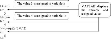
The result of entering a command is a variable with name ans. The equal sign (=) is called the assignment operator and is used to specify a value to a variable, e.g. to the ans. An entered new value cancels its predecessor.
Arithmetic operations are performed in the following order: operations in parentheses (starting with the innermost), exponentiation, multiplication and division, addition and subtraction. If an expression contains operations of the same priority, they run from left to right.
Examples of arithmetic operations in the Command Window are given below:
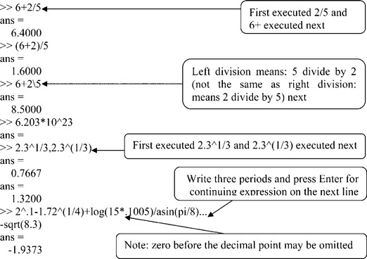
The outputted numbers are displayed here in short format (default format) – a fixed point followed by four decimal points. The format can be changed to long, 14 digits after the point, by typing the command: format long. To return to the default format the user has to type format.
There are other formats that can be obtained by typing help format; the word after help appears in blue, for ease of viewing.
2.1.3 Help and Help Window
For information about use of some commands, type and enter help with the command name after a space next to this word, e.g. help format as above. The explanations appear immediately after this in the Command Window. For a command concerning a particular topic of interest, the lookfor command may be used. For example, for the name of MATLAB® command(s) on the subject of codons one should enter lookfor codon and the commands will subsequently appear on the screen, as shown below:
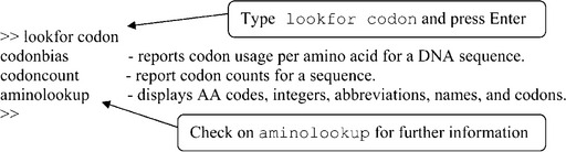
For further information the user has to click on the selected command or again use the help command. To interrupt the search process, the two abort keys Ctrl and c should be clicked together; these keys should also be used to interrupt any other process, e.g. that of program/command execution.
For more detailed information one can similarly use the doc command, e.g. doc aminolookup, in which case the Help window will be opened. The Help window can also be opened by selecting the Product Help line in the Help options on the MATLAB® Desktop menu line (Figure 2.4).
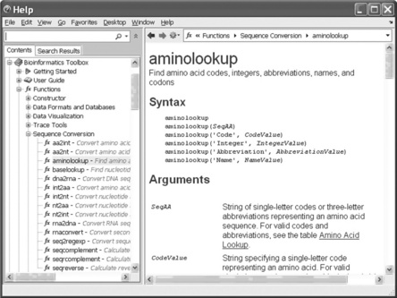
The Help window comprises three panes: on the left are the Contents or Search Results and on the right is the page containing information on the topic. Information on any subject is obtainable by typing the word(s) into the search line in the upper left-hand corner. The Search Results pane shows a preview of where the search words were found within the page, and the concrete information is displayed on the right.
2.1.4 Variables and commands for management of variables
A variable is a symbolic term written as a letter(s) and associated with a concrete numerical value. MATLAB® allocates memory space for storage of variable names and their values. A variable can be a scalar – a single number – or an array – a table of numbers. The name can be as many as 63 characters long, and contain letters, digits and underscores, but the first character must be a letter. Existing commands (sin, cos, sqrt, etc.) cannot be used as names.
The assignment and usage of variables in algebraic calculations is demonstrated next.
Predefined MATLAB® variables can be used without being assigned. Except for the previously mentioned pi and ans, these are inf (infinity), i or j (square root of − 1), and NaN (not-a-number, used when a numerical value is moot, e.g. 0/0).
The following commands can be used for management of variables: clear, to remove from memory; clear x y, for removing named variables x and y only; who for displaying the names of variables; or whos for displaying variable names, matrix sizes, variable byte sizes and variable classes. This information can also be obtained in the Workspace Window, where each variable is presented by the icon ![]() with the same information as in the case of whos but with additional data; the popup menu for selection of desirable information appears by right-clicking with the cursor placed on the Workspace Window menu line.
with the same information as in the case of whos but with additional data; the popup menu for selection of desirable information appears by right-clicking with the cursor placed on the Workspace Window menu line.
2.1.5 Output commands
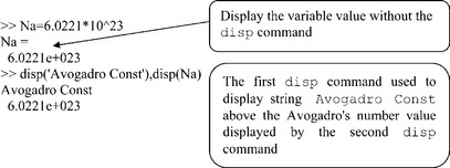
As previously noted, MATLAB® automatically displays the result after each command is entered, but does not display it if the command is followed by a semicolon. MATLAB® has additional display commands, the two most frequently used of which are disp and fprintf.
The disp command is used to display text or variable values without the name of the variable and the equal sign. Each new disp command yields its result in a new line. In general form the command reads
The text between quotes is displayed in blue.
The fprintf command is used to display text and data or to save them to file. The command has various forms that present difficulties for beginners, and here I give the simplest of them for displaying the results of a calculation.
To display text and a number on the same line the following form is used:
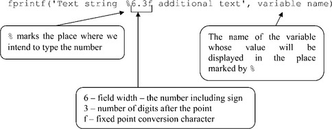
To divide a text into two or more lines, or starting with a new line, (slash n) must be written before the word or sign that we want to see on the new line. The field width and the number of digits after the point (6.3 in the example presented) are optional; the sign % and the character f, called conversion character, are obligatory. The character f specifies the fixed point notation in which the number is displayed. Some additional notations that can be used are: i, integer, e, exponential (e.g. 2.309123e + 001); and g, the more compact form of e or f, with no trailing zeros.
Addition of several %f units (or full formatting elements) permits inclusion of multiple variable values in the text. For example, using the fprintf command:
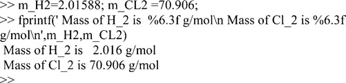
The color of the text in quotes is the same as in disp (blue).
The commands described can be used to output tables as will be shown later, after introduction of vectors and matrices.
2.1.6 Application examples
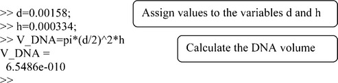
2.1.6.1 DNA volume
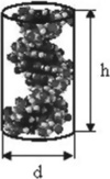
the idealized volume of the DNA molecule can be calculated using the expression for the volume of a cylinder:
where r, the radius of the DNA molecule, is about 1.58 × 10⁻³ μm, and h, its length, is 3.34 × 10⁻³ μm.
Problem: Calculate the volume of the DNA molecule.
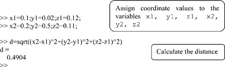
2.1.6.2 The distance between two molecules
The distance d between two molecules shown in a figure in a Cartesian coordinate system is given by the expression
where x, y and z are the coordinates, and subscripts 1 and 2 denote the first and second molecules, respectively. The dimensionless coordinates are: x1 = 0.1, y1 = 0.02, z1 = 0.12, x2 = 0.2, y2 = 0.5, z2 = 0.11.

Problem: Calculate the distance for the given coordinates of the molecules. The solution:
2.1.6.3 Cooling of a fluid according to Newton’s law
The time t taken for a liquid (e.g. coffee in a cup) to cool from temperature T0 to T is given from Newton’s law, according to
where Ts is the ambient temperature, T0 is the initial temperature and k is a constant. If the coffee has an initial temperature of 70 °C, the ambient temperature is 20 °C and k is 0.3 C/min.
Problem: When will the coffee be fit to drink (T = 28 °C)?
2.1.6.4 Constant of chemical reaction
The rate constant k of a chemical reaction is given by the Arrhenius equation:
where Ea is the activation energy, A is the frequency of molecular collision, T is the temperature at which the reaction passes and R is the gas constant. If for a dissociation reaction these parameters are Ea = 75,000 J/mol, A = 1 × 10¹⁴ s−1, T = 300 K and R = 8.314 J/(K mol), then the solution is:
2.2 Vectors, matrices and arrays
In the above, the single variables were used usually in scalar form. In MATLAB® this means that the variable is a 1 × 1 matrix. Two-dimensional matrices and arrays represent a numerical table, but mathematical operations with a matrix are applied in accordance with the rules of linear algebra, while arrays are used in element-wise operations.
2.2.1 Generation of vectors and matrices: vector and matrix operators
2.2.1.1 Generation of vectors
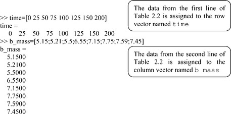
Vectors are presented as numbers written sequentially in a row or in a column, and termed, respectively, row or column vectors. They can also be presented as lists of words or equations. In MATLAB® a vector is generated by typing the numbers in square brackets with spaces or comma between them in the case of a row vector, and with semicolons between them, or by pressing Enter between them, in the case of a column vector.
The data for an aerobic biomass process as per Table 2.2 can be presented as two vectors, for example:
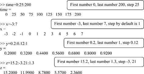
There are also two frequently used operators for generating vectors, namely (colon) and linspace.
The colon operator has the form
where i and k are respectively the first and last term in the vector and j is the step between the terms within it. The last number cannot exceed the last number k. The step for j can be omitted; in such a case it is equal to 1 by default. Examples are:
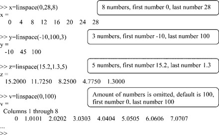
The linspace operator has the form
where a is the first number, b is the last number and n is the amount of numbers. When n is not specified, it takes the value of 100 by default.
The position of an element in a vector is its address; for example, the fifth position in the eight-element vector b_mass above can be addressed as b_mass(5), and the element located here is 7.15. The last position in the b_mass vector may be addressed with the end terminator; for example, b_mass(end) is the last position in the b_mass vector and assigns the number located here, 7.45; another way to address the last element is to give the position number, namely b_mass(8).
2.2.1.2 Generation of matrices and arrays
A two-dimensional matrix or an array has rows and columns of numbers and resembles a numerical table, the only difference being in realization of certain mathematical operations. When the number of rows and columns is equal the matrix is square, rectangular otherwise. Like a vector, it is generated by typing the row of elements in square brackets with spaces or commas between them and with semicolons between the rows, or by pressing Enter between the rows; the number of elements in each row should be equal.
The elements can also be variable names or mathematical expressions.
As an example, Table 2.3 presents repeated tests on three batches of enzyme activity:
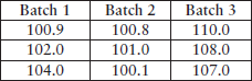
Matrix presentations of this table and other examples are:
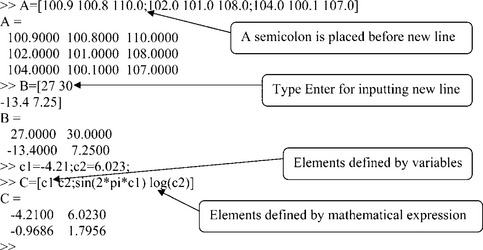
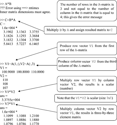
For manipulations with matrix elements, row–column addressing is used. For instance, in matrix A in the previous example set A(2,3) refers to the number 108.0000 and A(3,2) to the number 100.1000. Row or column numbering begins with 1, such that the first element in matrix A is A(1,1).
For sequential elements or an entire row or column, the semicolon can be used; for example, A(2:3,2) refers to the second and the third numbers in column 2 of matrix A, A(:,n) refers to the elements of all rows in column n and A(m,:) to those of all the columns in row m.
In addition to row–column addressing, linear addressing can be used. In this case a single number is used instead of the row and column numbers, and the element’s place within the matrix is indicated sequentially beginning from the first element of the first column and along it, then continuing along the second column and so up to the last element in the last column. For example, A(6) refers to element A(3,2), A(8) to A(2,3), A(4:6) is the same as A(:,2), etc.
Using square brackets, it is possible to generate a new matrix by combining an existing matrix with a vector or with another matrix.
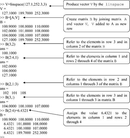
Examples of this kind of matrix manipulation are presented below, using matrix A from the previous example.
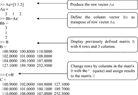
For conversion of a row/column vector into a column/row vector and for the rows/columns exchange in matrices, the transpose operator ' (quote) is applied, for example:
2.2.2 Matrix operations
Vectors, matrices and arrays can be used in various mathematical operations in the same way as single variables, as illustrated below.
2.2.2.1 Addition and subtraction
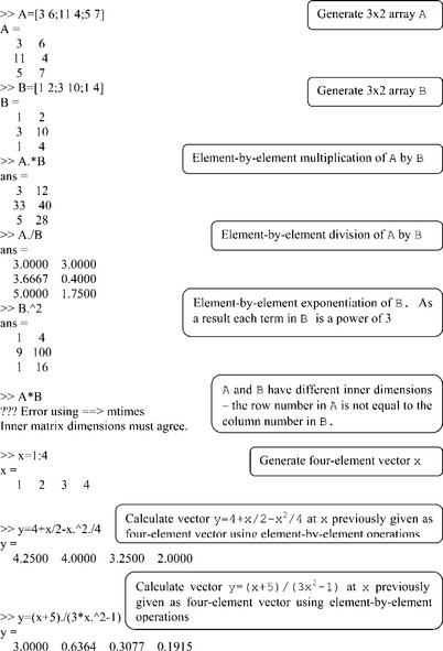
Addition and subtraction of two matrices are performed element by element, provided the matrices are equal in size; for example, when A and B are two matrices with size 3 × 2 each:
In addition and subtraction operations the commutative law is valid, namely A + B = B + A.
2.2.2.2 Multiplication
Multiplication of matrices is more complicated; in accordance with the rules of linear algebra, it is feasible only when the number of row elements in the first matrix equals to that of column elements in the second – in other words, the inner matrix dimensions must be equal. Thus the above matrices A, 3 × 2, and B, 3 × 2, cannot be multiplied, but if B is replaced by another with size 2 × 3, the inner matrix dimensions are equal and multiplication becomes possible.
It is not difficult to verify that the product B*A is not the same as A*B, and the commutative law does not apply here.
Various examples of matrix addition, subtraction and multiplication are given below, using the same A and B matrices as in the preceding section.
An important advantage of matrix multiplication is being able to present a set of linear equations in matrix form. For example, the set of two equations with two variables
may be written in compact matrix form as AX = B or in full matrix form as
2.2.2.3 Division
Division of matrices is even more complicated than their multiplication, as a result of the above-mentioned non-commutative properties of the matrix. A full explanation can be found in books on linear algebra. Here the related operators are described in the context of their usage in MATLAB®.
Identity and inverse matrices are often used in dividing operators. An identity matrix I is a square matrix whose diagonal elements are l’s and the remainder 0’s. It can be generated with the eye command (see Table 2.4 on p. 26). The commutative law applies – multiplication of A by I or I by A yields the same result: AI = IA = A.
Table 2.4
Commands for matrix manipulations, generation and analysis
| Form of MATLAB® presentation | Description | MATLAB® example (inputs and outputs) |
| length(x) | Returns the length of vector x | > > x = [3 7 1]; > > length(x) ans 31 |
| size(a) | Returns two-element row vector; the first element is the number of rows in matrix a and the second the number of columns. | > > a = [1 2; 7 3; 9 6]; > > size(a) ans = 3 2 |
| reshape(a,m,n) | Returns an m by n matrix whose elements are taken column-wise from a. Matrix a must have m*n elements | > > reshape(a,2,3) ans = 1 9 3 7 2 6 |
| strvcat(t1,t2,t3,…) | Generates the matrix containing the text strings t1, t2, t3, … as rows. | > > t1 = 'Alanine'; > > t2 = 'Arginine'; > > t3 = 'Asparagine'; > > strvcat(t1,t2,t3) ans Alanine Arginine Asparagine |
| zeros(m,n) | Generates an m by n matrix of all zeros | > > zeros(2,3) ans = 0 0 0 0 0 0 |
| diag(x) | Generates a matrix with elements of vector x placed along the diagonal | > > x = 1:3;diag(x) ans = 1 0 0 0 2 0 0 0 3 |
| eye(n) | Generates a square matrix with diagonal elements 1 and others 0 | > > eye(4) ans = 1 0 0 0 0 1 0 0 0 0 1 0 0 0 0 1 |
| randi(imax,m,n) | Returns an m by n matrix of integer random numbers from value 1 up to imax, the maximal integer value | > > randi(10,1,3) ans = 9 10 2 |
| b = min(a) | Returns row vector b with minimal numbers of each column in the matrix a. If a is vector, b is equal to the minimal number in a | > > a = [1 2; 7 3; 9 6]; > > b = min(a) b = 1 2 > > a = [1 2 7 3 9 6]; > > b = min(a) b = 1 |
| b = max(a) | Analogously to min but for maximal element | > > a = [1 2 7 3 9 6]; > > b = max(a) b = 9 |
| b = mean(a) | Returns row vector b with mean values calculated for each column of the matrix a. If a is a vector, returns average value of the vector a | > > a = [1 2; 7 3; 9 6]; > > b = mean(a) b = 5.6667 3.6667 |
| sum(a) | Returns row vector b with column sums of matrix a. Returns vector sum if a is a vector | > > a = [1 2; 7 3; 9 6]; > > sum(a) ans = 17 11 |
| std(a) | Analogously to sum but calculates standard deviation | > > a = [1 2; 7 3; 9 6]; > > std(a) ans = 4.1633 2.0817 |
| det(a) | Calculates determinant of the square matrix a | > > a = [5 6;12 1]; > > det(a) ans = − 67 |
| sort(a) | For vector or matrix. Sorts, respectively, elements of a vector or each column of a in ascending order. | > > a = [5 6;12 1;1 7]; > > sort(a) ans = 1 1 5 6 12 7 |
| num2str(a) | Converts a single number or numerical matrix elements into a string representation | > > a = 12.4356; > > num2str(a) ans = 12.4356 |
The matrix B is called the inverse of A when left or right multiplication leads to the identity matrix: AB = BA = I. The inverse matrix can be written as A−1. In MATLAB® this can be written in two ways: B = A^–1 or with operator inv as B = inv(A).
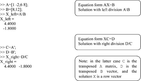
Where matrix products are involved, left, , or right, /, division is used. For example, to solve the matrix equation AX = B, with X and B column vectors, left division should be used: X = AB, while to solve XC = B, with X and B row vectors and C as the transposed matrix of A, right division should be used: X = B/C.
For example, we can use matrix division to solve the following set of equations:
According to the above, this set of equations can be represented in two matrix forms:
The solutions for both these forms are:
An application example with matrix division is given in Subsection 2.3.4.1.
2.2.3 Array operations
All previously described operations concern matrices obeying linear algebra rules; however, there are many calculations (in particular in bioscience) where the operations are carried out by the so-called element-by-element procedure. In these cases, to avoid confusion, we use the term ‘array’. These element-wise operations are carried out with elements in identical positions in the arrays. In contrast to matrix operations, element-wise operations are confined to arrays of equal size; they are denoted with a point typed preceding the arithmetic operator, namely .* (element-wise multiplication); ./ (element-wise right division), . (element-wise left division) and .^ (element-wise exponentiation).
For example, if we have vectors a = [a1 a2 a3] and b = [b1 b2 b3] then element-by-element multiplication a. *b, a. /b and exponentiation a. ^b yields:
The same manipulations for two matrices  and
and  lead to:
Element-wise operators are frequently used to calculate a function at series of values of its argument. Examples of array operations are:
2.2.4 Commands for generation of special matrices and some additional commands for matrices and arrays
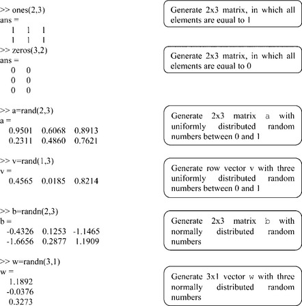
There are also some commands for generating matrices with special values and those with random values. The ones(m,n) and zeros(m,n) commands are used for matrices of m rows and n columns with 1 and 0 as all elements. Various practical problems involve random numbers, for which the rand(m,n) or randn(m,n) command should be used, the former yielding a uniform distribution of elements between 0 and 1 and the latter a normal one with mean 0 and standard deviation 1. The randseq command, which generates random DNA, RNA and amino-acid sequences, is explained in Chapter 7. For generating a square matrix (n × n), these commands can be abbreviated to rand(n) and randn(n). Examples are:
Integer random numbers can be generated with the randi-command as shown in Table 2.4.
In addition to the commands described in the previous sections, MATLAB® has many others that can be used for manipulation, generation and analysis of matrices and arrays; some of these are listed in Table 2.4.
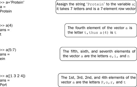
All matrices described above had numerical elements even if they have the expressions as an element because these expressions yield numbers, when evaluated. But as a single element or number of elements of a matrix, a string(s), can be used. A string is an array of characters – letters and/or symbols. A string is entered in MATLAB® between single quotes, e.g. ‘Protein’ or ‘Human cells DNA < deoxyribonucleic acid > totals about 3 meters in length’. Each character of the string is presented and stored as a number (thus the set of characters represents a vector or an array) and can be addressed as an element of a vector or array, e.g. a(5) in the string ‘Protein’ is the letter ‘e’. Some examples with string manipulations are:
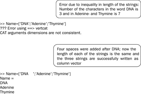
Strings can be placed as elements in a vector or a matrix. String rows are divided the same as numerical rows by a semicolon (;) and strings within the rows by a space or a comma. Rows should have the same number of elements and each column element must be the same length as the longest of the column elements. To achieve this alignment, spaces should be added to shorter strings; for example
2.2.5 Application examples
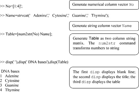
2.2.5.1 DNA bases table
DNA has four bases, adenine, cytosine, guanine and thymine.
Problem: Generate and display the matrix in which the first column is the serial number and the second is the base name.
Make it in the following steps:
• Generate a numerical column of values from 1 to 4.
• Generate a string column with the names adenine, cytosine, guanine and thymine.
• Join these two columns in to a matrix. In MATLAB® all matrix elements should be of the same type; for example, if strings are written in one column, then another column must also contain strings or vice versa – in our case we use the num2str command, which transforms numerical data into string data.
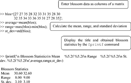
2.2.5.2 Blossom statistics
A biotech company has developed a new type of fruit tree. Below are blossom yield data from ten trees, checked twice at different times, and presented in two rows (time) and in ten columns (trees):
Problem: Find the mean, the difference between maximal and minimal values (range), and the standard deviation for every row of the data, and display the results to two decimal places, using the fprintf command.
• The tree blossom data are assigned to a two-row matrix.
• The mean, range and standard deviation are calculated by the appropriate MATLAB® commands.
• The statistics obtained are displayed via the fprintf command.
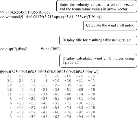
2.2.5.3 Wind chill index
Wind chill w is the apparent temperature experienced at wind velocity v and air temperature T. An empirical formula for it is:
where w is in degrees Fahrenheit, v is in m/s (4, 5, 10, 15, 20, 25, 30, 35, 40 and 45) and T decreases from 35 to − 35 at steps of 10°, also in Fahrenheit.
Problem: Write the command for the wind chill matrix by giving vectors v and T and display it as a table, so that w is arranged along the rows at constant v and along the columns at constant T.
• Generate separately the column-vector v (size 10 × 1) and the row- vector T (size 1 × 8).
• Calculate the w-matrix according to the formula. The first multiplier (the terms in the first set of parentheses of the w-expression) has size 10 × 1 and the second (the terms in the second set of parentheses) has size 1 × 8, and thus their product according to linear algebra would be size 10 × 8 (extreme values of the sizes of these vectors).
• Display the title ‘Wind chill’ and w-matrix with the digits that are before the decimal point only.
The commands to the solution are:
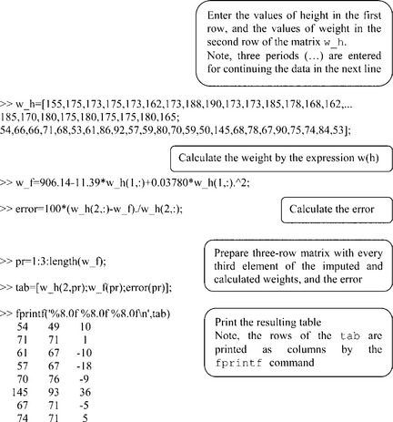
2.2.5.4 Weight versus height
Measurements of students’ weight w (in kg) and height h (in cm) in a group at an American college showed the following results: heights – 155, 175, 173, 175, 173, 162, 173, 188, 190, 173, 173, 185, 178, 168, 162, 185, 170, 180, 175, 180, 175, 175, 180, 165; weights – 54, 66, 66, 71, 68, 53, 61, 86, 92, 57, 59, 80, 70, 59, 50, 145, 68, 78, 67, 90, 75, 74, 84, 53. These data were fitted by the polynomial expression
Problem: Write the commands to input data in a two-row matrix, w_h, and calculate the weight by the expression and the percentage error, 100(w – wf)/w. Display the results as a three-column table listing every third value of w, wf and the error.
• The height and weight values are assigned as above.
• The weights wf and the errors are calculated according to the described expressions.
• Every third value of the input and calculated values of weight, and the calculated errors, are written in a three-row matrix tab and displayed as a three-column table.
2.3 Flow control
A calculation program represents a sequence of commands implemented in a given order. However, there are many cases when the written order of single – or group of – commands should be altered, for example when a calculation should be repeated with new parameters, or when one of several expressions has to be chosen to calculate a variable. For example, bacterial growth proceeds in four phases, lag, log, stationary and death, for each of which a different expression should be used to calculate population size. Another example is provided by DNA, RNA and protein sequence analyses, where the alignment procedure is repeated until the best matching score is reached.
Flow control is applied in such processes. In MATLAB®, special commands, usually called conditional statements, are used for these purposes; by this method the computer decides which command should be carried out next. The most frequent flow control commands are described below.
2.3.1 Relational and logical operators
Relational operators. Operators matching a pair of values are called relational or comparison operators; the application result of such an operator is written as 1 (true value) or 0 (false value) – for example, the expression x < 3 results in 1 if x is less than 3 and in 0 otherwise.
The relational operators are: < (less than), > (more than), <= (less than or equal to), > = (more than or equal to), = = (equal to) and ~ = (not equal to). Two-sign operators should be written without spaces.
Where a relational operator is applied to a matrix or an array, it performs element-by-element comparisons. This returns an array of ones where the relation is true (the array has the same size as the size of the matrices compared), and zeros where it is not. If one of the compared objects is scalar and the other a matrix, the scalar is matched against every element of the matrix. The ones and zeroes are logical data and are not the same as numerical data, although they can be used in arithmetical operations.
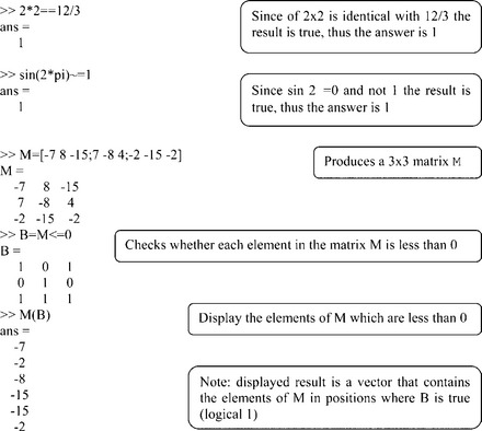
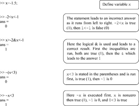
Logical operators. Logical operators are designed for operations with the true or false values within the logical expressions. They can be used as addresses in another vector, matrix or array.
In MATLAB® there are three logical operators: & (logical AND), | (logical OR) and ~ (logical NOT). Like the relational operators they can be used as arithmetical operators and with scalars, matrices and arrays. Comparison is element-by-element with logical 1 or 0 when the result is true or false, respectively. MATLAB® also has equivalent logical functions: and(A,B), equivalent to A&B, or(A,B), equivalent to A|B, and not(A,B), equivalent to A ~ B. If the logical operators are performed on logical variables the results will follow Boolean algebra rules. In operations with logical and/or numerical variables the results are logical 1 or 0.
Another MATLAB® logical function is find, which in it simplest forms reads as
where i is a vector of elements which are non-zero (first case), or belong to a vector A and are larger than c (second case); for example, vector v = [12 0.1 3.4 0–2.5], and thus
Note: any relational operator(s) can be written in the find command, e.g. find(A < 0.5), or find(A > = 9). The order in which combinations of relational, logical and conditional operators is executed (so-called precedence rules) is obtainable in advanced MATLAB® courses. The order of execution of such an operator can also be annotated using parentheses.
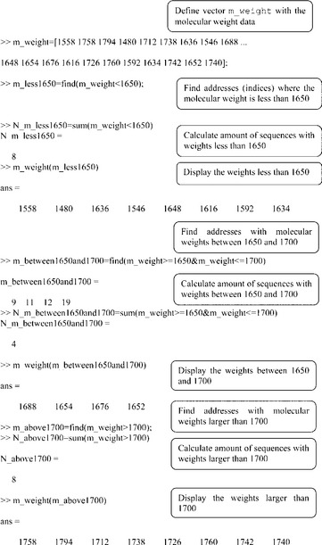
2.3.1.1 Application example: molecular weight screening
The molecular weights of 20 randomly generated sequences comprising 20 letters of the DNA alphabet are 1558, 1758, 1794, 1480, 1712, 1738, 1636, 1546, 1688, 1648, 1654, 1676, 1616, 1726, 1760, 1592, 1634, 1742, 1652 and 1740.
Problem: Use relational and logical operators to determine the number of sequences with molecular weight (a) less than 1650, (b) between 1650 and 1700, and (c) more than 1700. Display the molecular weights for each of these groups. The commands that solved this problem are presented on p. 37.
2.3.2 If statements
In program flow control, various conditional statements are widely used. The first of them is the if statement, which has three forms: if … end, if … else … end, and if … elseif … else … end. Each if construction terminates with the word end; its words appear on the screen in blue.
The if statements are shown in Table 2.5.
Table 2.5
| if … end | if … else … end | if … elseif … else … end |
| if conditional expression MATLAB® command(s) end |
if conditional expression MATLAB® command(s) else MATLAB® command/s end |
if conditional expression MATLAB® command(s) elseif conditional expression MATLAB® command(s) else MATLAB® command(s) end |
In conditional expressions the relational and logical operators are used, for example a < = b&a > = c or b = = c.
When the if with a conditional expression is typed next to the prompt > > and Enter is pressed, the next (and each additional) line appears without the prompt until the word end is typed.
An application example in which the if statement is used is presented at the end of Section 2.3.
2.3.3 Loops in MATLAB®
Another method of program flow control is a loop, which permits a single command, or a group of commands, to be repeated several times. Each
cycle of commands is termed a pass. There are two loop commands in MATLAB®: for … end and while … end. These words appear on the screen in blue. As with if statements, each for or while construction should terminate with the word end.
The loop statements are written in general form in Table 2.6.
Table 2.6
| for … end loop | while … end loop |
| for k = [initial : step : final] MATLAB® command(s) end |
While conditional expression MATLAB® command(s) end. |
In for … end loops the commands written between for and end are repeated k times, a number which increases for every pass by addition of the step-value; this process is continued until k reaches or exceeds the final value.
The square brackets in the expression for k (Table 2.6) mean that k can be assigned as a vector, for example k = [3.5 –1.06 1:2:6]. The brackets can be omitted if there are only colons in k, e.g. k = 1:3:10. The last pass is followed by the command next to the loop. For some calculations realized with for … end loops matrix operations can serve as well. In such cases the latter are actually superior, as the for … end loops work slowly. The advantage is negligible for short loops with a small number of commands, but is appreciable for large loops with numerous commands.
The while … end loop is used where the number of passes is not known in advance and the loop terminates only when the conditional expression is false. In each pass MATLAB® executes the commands written between the while and end; the passes are repeated until the conditional expression is true. An incorrectly written loop may continue indefinitely; for example,
In this case the expression a = Inf appears repeatedly on the screen. To interrupt the loop, the Ctrl and C keys should be pressed together.
Examples of the for … end and while … end loops used for calculating ex via the series  at x = 2.3 are (see p. 39):
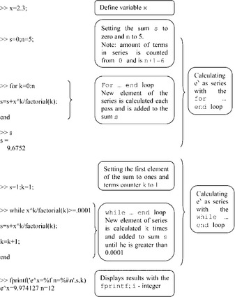
In the for … end loop the sum s is calculated; at the start of the first pass s = 0, and during this pass the first term (k = 0) is calculated and added to s. On the second pass k = k + 1 = 1, the second term of the series is calculated and added to s. This procedure is repeated up to k = n (n = 5 in this example). After this the loop ends and the value obtained is displayed after entering the variable name s. The number of passes is fixed in for … end loops. In situations where the while … end loop is used, a condition for loop ending must be given. A value of the kth term larger than 0.0001 was taken for this. With the start of the first pass the value of s is equal to a value of the first term of the series (k = 0, x0/0! = 1) and k is equal to 1 (k in this case is called counter), and these values are assigned before the loop. In the first pass the second term of the series is calculated and added to the sum s, and the value of k is increased by 1. If the condition is true the next pass is started and the next term calculated; if it is false, the loop is ended and the fprintf command displays the value of s obtained and number of terms used – if the latter value is an integer then a conversion character i is used to display the value of k.
For … end and while … end loops and if statements can be included in other loops, in if statements, or one into another. There is no limit to the number of such inclusions.
2.3.4 Application examples
2.3.4.1 Compound concentration and the instrument response
An instrument used in a biotechnology laboratory has a response R with values 0.31, 0.43, 0.70, 1.1, 1.5, 1.79 and 2.2 to the following compound Z concentrations, c: 100, 150, 250, 400, 550, 650 and 850 mg/mL. The best linear fit equation c = a1 + a2R is obtainable by solving the set
where n is the number of (R,c) points.
This set can be represented in matrix forms AX = B or XA = B, in our case:
Problem: Define the a-coefficients with left- and right divisions; the result can be printed as a linear equation with the relevant coefficients a1 and a2.
The steps to be taken are as follows:
• Generate two row vectors with the given R and c values;
• Generate a 2 × 2 matrix A with the sums on the left-hand side of the first matrix forms; for sums the sum command can be used;
• Generate a column vector B with the sums on the right-hand side of the first matrix equation;
• Use the left division AB for calculation of the a-coefficients;
• Display with the fprintf command the coefficients in the written linear equation;
• Resort to the right division AB. For this A should be written as per the second matrix equation, using the quote operator (‘). The letter serves to transform the column vector B into the row vector; the right division in this case is simply verification of the previous solution.
• Display with the fprintf command the coefficients directly in the written linear equation.
The commands for solution are:

2.3.4.2 Bacteria population growth
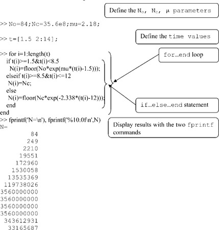
Changes in a bacteria population of size N (cells/mL) were measured from t0 = 1.5 up to 14 (hours). The results obtained were fitted by the following expressions:
where t is time in hours, N0 is the initial bacteria population at time t0, Nc is the population in the stationary phase, μ is the growth rate constant (h−1), floor means that bacteria number should be an integer; the parameters required are: N0 = 84, Nc = 35.6 × 10⁸ and μ = 2.18.
Problem: Calculate bacteria populations at 1.5, 2, 3, …, 14 hours.
• Determine the variables N0, Nc and μ, and a 1 × 14 vector with the t values;
• Use the for… end loop in which every pass runs for the new t value defined by its index (address) – t(i);
• Introduce in the loop the statement if … elseif … else … end in which the conditions and expressions on the right-hand side of the equation defining N should be written in the blank spaces; the values of N should be indexed to generate the vector of calculated N-values for each t;
• Display with the fprintf the vector of calculated N-values.
The commands for calculating N are
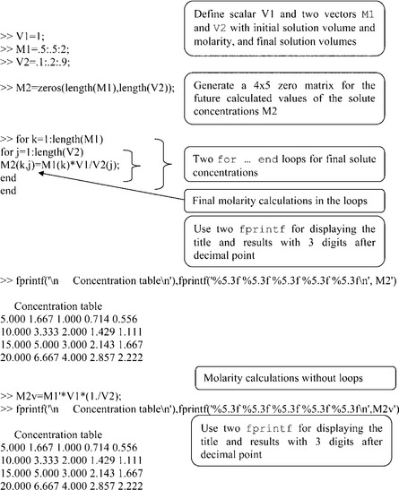
2.3.4.3 Dilution
The resulting molar concentration of a solution, M2, is calculated via
where V2 is final solution volume, and M1 and V1 are the initial concentration and solution volume, respectively.
A series of standard solutions were prepared with M1 values of 0.5, 1, 1.5 and 2 mol/L and common V1 values of 0.1 L.
Problem: Calculate the table of molar concentrations M2 if each of the prepared series of standard solutions was diluted by 0.1, 0.3, 0.6 and 0.9 L of water.
This can be constructed in two ways – using for… end loops and without the loops using the vectors for V2 and M1 only.
The required steps are as follows:
• Enter the value of V1 and generate vectors for M1 and V2;
• Generate a matrix with the number of rows equal to the length of the M1 vector and that of columns equal to the length of the V2 vector; this step pre-allocates the matrix and serves to reduce operation time when the for … end construction is used (a minor consideration for small matrices but quite significant for large ones);
• Calculate M2 (with the expression above) in the two for … end loops: the external for M1 and the internal for V2; such a construction yields all values M2 for each V2;
• Display the calculated matrix M2 with the fprintf, in which the values obtained are presented with three digits after the decimal point.
• Repeat the same calculations but without loops; for this rewrite the expression in the form M1V1(1/V2) so that the element-wise division in brackets comes first and is followed by the multiplication; (1/V2) produces a row vector with size 1 × 4 and for the inner dimension equality the vector M1 should be transformed by the quote operation (') to a column vector with size 4 × 1; the next multiplication by the scalar V1 does changes the vector size, and the product of the [4 × 1]*[1 × 5] matrices is the final 4 × 5 matrix with the calculated M2 values.
2.4 Questions for self-checking and exercises
1. Which command should be used to list the names of variables in the workspace? Choose from: (a) lookfor, (b) whos, (c) who.
2. The predefined variable π with format long is displayed as: (a) 3.1416, (b) 3.14, (c) 3.141592653589793, (d) 3.141592653589793e + 000?
3. Which of the MATLAB® expressions below is suitable for the equation 
4. The command M = [1;2;3;4] generates (a) a row vector, (b) a column vector or (c) a square matrix?
5. Which of the next special commands generates the matrix  :
:
6. The command that generates uniformly distributed integer random numbers is: (a) rand, (b) randn or (c) randi?
7. Which of the answers below is correct for the division [2 4;6 8]/[1 2;3 4]:
8. For transformation of a row vector T with numerical values into a column vector, the following MATLAB® expression should be written:
9. To address the element in a 3 × 3 matrix A located at the third row and the second column, the following MATLAB® expression should be written:
Note: More than one correct answer is possible.
10. With some idealization, the corpuscle of muscle hemoglobin can be treated as a sphere 20 microns in diameter. Calculate its volume with the expression
11. The mass flow rate (L/min) of blood in the human circulatory system can be calculated by the empirical expression
where m = mass in kg and h = height in m. Calculate the mass flow rate in men with parameters m = 80 kg and h = 1.8 m.
12. The temperature distribution in a biological system containing blood vessels is described by the expression
Calculate the temperature at r = (a + b)/2 when a = 0.5, b = 0.65, Ta = 315 and Tb = 310.
13. The velocity v of molecules in the Cartesian coordinate system is represented via its coordinate components vx, vy and vz by the equation
Calculate the velocity for vx, vy and vz = 2.1, –3.1 and 0.72, respectively.
14. The decay process of radioactive substances with time is described by the equation
where t is the number of half-life periods elapsed (the half-life being the time it takes for a decaying substance to disintegrate by half), N0 is the initial amount of the substance and N is the residual amount.
(a) Calculate N for t = 0, 8, 16 and 24 days for substances with N0 = 500 μCi (microCuries).
(b) Display the data as a two-column table, the first column t and the second N.
15. The Fourier series is one of the best instruments for description of complex biological shapes; the first terms in these series can be obtained as
Calculate F for coefficients a1 and b1 of 1.2 and 0.7, respectively, phase angles ψ1 and ψ2 of 0.1 and 0.2, respectively, and x = π/7.
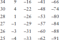
16. The molecular weights (g/mol) for ten amino acids are given in the table
![]()
(a) Generate a Name vector with acid name notations;
(b) Generate a Weight vector with molar weight values;
(c) Generate a 10 × 2 matrix in which the first column are the Names and the second the Weights; use the num2str command for string representation of values in the matrix columns;
17. Use the table in Exercise 16 to list those amino acids with molecular weights (a) less than 100, (b) between 100 and 150, and (c) more than 150. Display the results in such a form that the title appears for each group and then each row shows the amino acid name and molecular weight; use the disp commands.
18. The wind chill index can be calculated by the expression
in which the wind velocity v (mph) takes values from 10 to 60 in steps of 10 mph and the air temperature T (F) from 40 to − 40 in steps of 20 °F.
(a) Calculate w for each of the given values of v and T using the for … end statements;
(b) Display the results with the fprintf command showing only integer values (digits preceding the decimal point only).
19. Calculate the wind chill index using the above expression without for … end statements, using vectors only. Note that the first term on the right-hand side of the equation for w represents a vector product and should generate a matrix – it cannot be summed with the vector represented by the second term as the vector and matrix differ in size and should be aligned; use the ones command.
20. In a laboratory the number of bacterial cells was measured every hour from 0 up to 7 hours; the results were 100, 200, 400, 800, 1600, 3200, 6400 and 12 800.
(a) Generate a vector t with the elapsed time data;
(b) Generate a vector N with the numbers of bacterial cells;
(c) Generate and display an 8 × 2 matrix in which the first row represent t and the second N;
(d) Determine the minimal and maximal values for the bacterial growth data;
(e) Determine the integer mean value for the bacterial cells data, using the round command;
(f) Calculate the range r as the difference between the maximal and minimal values of the number of bacterial cells;
(e) Display all the results with a single fprintf command, so that each value appears on a new line with its nomenclature (e.g. Average = 3187).
21. Weather conditions have a strong influence on mosquito populations. For example, an experiment has shown that at monthly rainfall q of 2, 7, 11, 18 and 23 mm the mosquito density d (average monthly number of mosquitoes trapped by all mosquito monitoring stations) was 0.8, 2.1, 4, 4.9 and 5.7, respectively. These data can be described by the linear equation q = a1 + a2d in which the coefficients a1 and a2 are obtainable from the following set of equations