
Ordinary and partial differential equation solvers
Differential equations play an important role in science and technology in general and in bioscience and bioengineering in particular. Many processes and phenomena in biokinetics, biomedicine, epidemiology, pharmacology, genetics and other life sciences can be described by such equations. They are often not solvable analytically, in which case a numerical approach is called for, but a universal numerical method does not exist. For this MATLAB® provides tools, called solvers, for solutions to two groups of differential equations – ordinary, ODEs, and partial, PDEs. The corresponding groups of solvers, ODEs and PDEPEs, are described in brief below. Basic familiarity with ordinary and partial differential equations is assumed.
5.1 Solving ordinary differential equations with ODE solvers
These solvers are intended for single or multiple ODEs of first order, having the form:
where n is the number of first-order ODEs, y1, y2, …, yn are the dependent variables and t is the independent variable; instead of t the variable x can also be used. In the case of high-order ODEs, they should be reduced to first order by creating a set of such equations. For example, the equation
 should be rewritten as a set of two first-order ODEs:
  Nevertheless, among practical life science problems, first-order ODEs predominate and thus solution of such equations is discussed further.
Table 5.1 on p. 135 lists the available solvers in MATLAB®, the numerical method each solver uses and the class of problem associated with each solver. These solvers are intended for so-called initial-value problems, IVPs, when the differential equation is solved with any initial value of the function, e.g. y = 0 at t = 0 for the equation 

The methods used in those solvers are based on finite differences by which the differential is presented:  which is apparently true for very small, but finite (non-zero) distances between the points; i here is the point number in the [a,b] range of the argument t. Giving the first-point value y0 at t0 and calculating the value of
  we get the next y1. Calculating
  for the next argument t1 we get y2 and the process is repeated until all function values in the range are available. This approach, originally realized by Euler, is used with different improvements and complications, and is used in modern numerical methods such as those of Runge–Kutta, Rosenbrock and Adams.
The class of problems associated with ODE solvers comprise three categories, namely non-stiff, stiff and fully explicit. There is no universally accepted definition of stiffness for the first two categories. A stiff problem is one where the equation contains some terms that lead to such variation as to render it numerically unsolvable even with very small step sizes, and the solution does not converge. In some cases, a rule for categorization of stiff ODEs is that the ratio of the maximal and minimal eigenvalues of the ODE is large, say 100 or more. Unfortunately, this criterion is not always correct and therefore it is impossible to determine in advance what ODE solver should be used for identification of the stiffness of an ODE. In contrast to stiff ODEs, an important feature of a non-stiff equation is that it is stable and the solution converges. Sometimes the stiff category of ODEs may be known in advance, for example from some physical reasons (e.g. a fast chemical reaction), but if the category is not known the ode45 solver is recommended first, and the ode15s next.
When an equation cannot be presented in explicit form ![]() and has the implicit form
and has the implicit form ![]() the ode15i solver is used. Implicit equations are rarely found in bio-problems and need not be discussed further here.
the ode15i solver is used. Implicit equations are rarely found in bio-problems and need not be discussed further here.
5.1.1 MATLAB® ODE solver form
The simplest command used in all ODE solvers has the form:
[t,y] = odeN(@ode_function,tspan,y0)
where odeN is one of the solver names, e.g. ode45 or ode15s; @ode_ function is the name of the user-defined function or function file where the equations are written. The function definition line should have the form
function dy = function_name(t,y).
In the subsequent lines of this file the differential equation(s), presented as described above in Subsection 5.1, should be written in the form
dy = [right side of the first ODE;right side of the second ODE; …]
tspan – a row vector specifying the integration interval, e.g. [1 12] – specifies a t-interval from 1 to 12; this vector can be given with more than two values for viewing the solution at values written in this vector; for example, [1:2:11 12] means that results lie in the t-range 1–12 and will be displayed at t-values of 1, 3, 5, 7, 9, 11 and 12; the values given in tspan affect the output but not the solution tolerance; as the solver automatically chooses the step for ensuring the tolerance, the default tolerance is 0.000001 absolute units.
y0 is a vector of initial conditions; for example, for the set of two first-order differential equations with initial function values y1 = 0 and y2 = 4, y0 = [0 4]. This vector can be given also as column, e.g. y0 = [0;4].
The odeN solvers can be used without the t and y output arguments; in this case the solver automatically generates a plot.
5.1.1.1 The steps of ODE solution
The solution of an ODE can be presented in the following steps:
1. As a first step, the differential equation should be given in the form
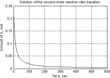
As an example we solve the rate equation of a unimolecular second- order reaction
where [A] is the amount of the reactant A, t is the time of the studied reaction, k is the reaction rate constant – say, k = 0.5 mol–1 s–1, the initial amount of A = 0.25 mol and t = 0–10 min.
This equation has an analytical solution, but here we consider a numerical solution. For this the equation should be rewritten in the form
2. Now the function file with the user-defined function containing dy/dt as function of t and y should be created. This file must be written in the Editor Window and then saved with a name given to the written function. For our example the function is
Therefore, the m-file containing this function is named ODEfirst.
3. In this step the solution method and appropriate ODE solver should be chosen from Table 5.1. In the absence of a specific recommendation, the ode45 solver for non-stiff problems will serve. The following command should be entered in the Command Window
> > [t,y] = ode45(@ODEfirst,[0:100:600], 0.25) % t = 0…600 sec, step 100; y0 = 0.25
The process starts at t = 0 and ends at t = 10 × 60 = 600 s, the initial value of y = 0.25 mol. It yields numbers but does not plot the results. To achieve both, the starting, ts = 0, and finishing, tf = 600, time values only may be given in tspan [which uses a default t-step and adds y(t) points for plotting]; and then the command for plotting should be entered:
> > [t,y] = ode45(@ODEfirst,[0 600], 0.25); % t = 0 …600 s with default step
> > xlabel(‘Time, sec’),ylabel(‘Amount of A, mol’)
> > title(‘Solution of the second order reaction rate equation’)
The generated plot (Figure 5.1) is:
 with A0 = 0.25.
To create a program with all commands included, the function file should be written. For the studied example, this file – named SecOrdReaction – reads as follows:
function t_A = SecOrdReaction(ts,tf,y0,n)
% Solution of the ODE for second order reaction rate
% t – time, sec; y – amount of the A-reactant, mol
% n- number of points for displaying
% To run:> > t_A = SecOrdReaction(0,600,0.25,5)
close all % closes all previously plotted figures
[t,y] = ode45(@ODEfirst, tspan, y0);
xlabel(‘Time, sec’),ylabel(‘Amount of A, mol’)
title(‘Solution of the second order reaction rate equation’)
t_n = linspace(ts,tf,n);% n t points for displaying
The input parameters in the written function are: tspan – time range, y0 – initial value of y and n – the number of points for displaying results, which should be greater than 2 but below the length of the vector t. The output parameter is the two-column matrix t_A with t in the first column and the amounts of A in the second. The n time-values t_n are generated by the linspace command, and the n concentrations y_n interpolated by the interp1 command; this is necessary because the number of t,y values calculated by the ode45 command and the desired number of these values can differ.
To run this file the following command should be typed and entered in the Command Window:
> > t_A = SecOrdReaction(0,600,0.25,5)
| 0 | 0.2500 |
| 150.0000 | 0.0127 |
| 300.0000 | 0.0065 |
| 450.0000 | 0.0044 |
| 600.0000 | 0.0033 |
The graph [A] = f(t) is also plotted by the SecOrdReaction function.
5.1.1.2 Extended form of the ODE solvers
When ODE solver commands are used for equations with parameters (e.g. in the discussed example the reaction rate constant k is a parameter), a more complicated form is necessary:
[t,y] = odeN(@ode_function,tspan,y0,[ ], param_name1,param_name2,..)
where [ ] is an empty vector; in the general case it is the place for various options that change the process of integration;1 in most cases, default values are used which yield satisfactory solutions and we do not use these options. param_name1, param_name2,… are the names of the arguments that we intend to write into the ode_function.
If the parameters are named in the odeN solver, they should also be written into the function.
For example, the SecOrdReaction file should be modified to introduce the coefficient k as an arbitrary parameter:
function t_A = SecOrdReaction(k,ts,tf,y0,n)
% Solution of the ODE for second order reaction rate %
k – reaction rate constant, 1/(mole sec)
% t – time, sec; y – amount of the A – reactant, mol
% n – number of points for sisplaying
% To run:> > t_A = SecOrdReaction(0.5,0,600,0.25,5)
close all % closes all previously plotted figures
[t,y] = ode45(@ODEfirst, tspan, y0,[],k);
xlabel(‘Time, sec’),ylabel(‘Amount of A, mol’)
title(‘Solution of the second order reaction rate equation’)
t_n = linspace(ts,tf,n);% n time points for displaying
y_n = interp1(t,y,t_n,’spline’);% n concentr. points for displaying
And in the Command Window the following command should be typed and entered:
> > t_A = SecOrdReaction(0.5,0,600,0.25,5)
The results are identical to those discussed above.
The advantage of the form with parameters is its greater universality; for example, the SecOrdReaction function with parameter k can be used for any second-order reaction with previously obtained reaction rate constant.
5.1.2 Application examples
The commands in the examples below are written mostly as functions with parameters. The single help line in these functions consists of a command that should be typed in the Command Window. In the general case the explanations for input and output parameters are conveniently introduced as described in the preceding chapter.
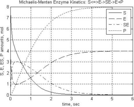
5.1.2.1 Michaelis-Menten kinetics
The enzyme-catalyzed reactions E + S![]() ES → E + P studied by Michaelis and Menten are described by the following set of four ODEs:
ES → E + P studied by Michaelis and Menten are described by the following set of four ODEs:
where [S], [E], [ES] and [P] are the amounts of substrate, free enzyme, substrate-bound enzyme and product, respectively, k1 and k1r are the direct and reverse reaction rate constants in the E + S![]() ES reaction, and k2 is the rate constant of the ES → P reaction.
ES reaction, and k2 is the rate constant of the ES → P reaction.
Problem: Solve the set of ODEs in the time range 0–6 s with initial [S] = 8 mol, [E] = 4 mol, [ES] = 0 and [P] = 0. Reaction rate constants are: k1 = 2 mol–1 s–1, k1r = 1 s- 1 and k2 = 1.5 s–1. Plot the component amounts as a function of time, and display the data obtained.
Formulate the set of equations in the form suitable for the ODE solver:
at 0 ≤ t ≤ 6 with k1 = 2, k1r = 1, k2 = 1.5 and initial y1 = 8, y2 = 4, y3 = 0 and y4 = 0.
Now, the ODE solver should be chosen. In the absence of preliminary reasons, the ode45 solver should be adopted.
The function file for the solution is
function t_S_E_ES_P = MichaelisMenten(k1,kr1,k2,ts,tf,S0,E0,ES0,P0,n)
% To run > > t_S_E_ES_P = MichaelisMenten(2,1,1.5,0,6,8,4,0,0,10)
[t,y] = ode45(@MM,tspan,[S0,E0,ES0,P0],[],k1,kr1,k2);
title(‘Michaelis-Menten Enzyme Kinetics: S < = > E- > SE- > E + P’)
xlabel(‘Time, sec’),ylabel(‘S, E, ES, P amounts, mol’)
t_n = linspace(ts,tf,n);% n time points for displaying
y_n = interp1(t,y,t_n,’spline’);% n concentrations for displaying
function dc = MM(t,y,k1,kr1,k2)
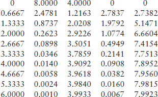
The input arguments in the MichaelisMenten function: k1, kr1, k2, S0, E0, ES0 and P0 correspond to k1, k1r, k2, [S]0, [E]0, [ES]0 and [P]0 in the original set; the tspan is a two-element vector with starting and end values of t; n, as in the preceding example, is the number of t,y-rows to be displayed.
The t_S_E_ES_P output argument is a five-row matrix with t and [S], [E], [ES] and [P] as the component amounts. As in the preceding example, the linspace and interp1 commands are used to display the n-rows of desired times t_n and accordingly the concentrations y_n.
To run the function in the Command Window, the following command should be typed and entered:
> > t_S_E_ES_P = MichaelisMenten(2,1,1.5,0,6,8,4,0,0,10)
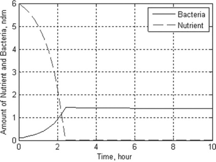
5.1.2.2 Chemostat
A chemostat2 is a container of volume V with constant culture medium inflow F and fresh nutrient concentration R. The differential equations for the concentration of bacteria N and that of nutrient S are:
where D = F/V is the dilution rate, r is the maximal growth rate, a is the half-saturation constant and γ is growth yield; square brackets [ ] denote concentration.
Problem: Solve the set of ODEs in the time range 0–10 s with r = 1.35 h–1, a = 0.004 g/L, D = 0.25 h–1, [R] = 6 g/L, γ = 0.23, [N]0 = 0.1 g/L and [S]0 = 6 g/L. Plot the nutrient and bacteria concentrations as a function of time, and display the data obtained.
Formulate the set of differential equations in the form suitable for the ODE solvers:
where y1 is [N] and y2 is [S], t is varied between 0 ≤ t ≤ 6, k1 = 2, k1r = 1, k2 = 1.5 and the initial y1 = 6 and y2 = 0.1.
The ODE solver should now be chosen; as the chemostat problem is stiff, the ode15s solver should be used.
The chemostat function file that solves the problem is:
function t_N_C = chemostat(r,a,gam,D,R,ts,tf,N0,S0,n)
%To run:> > t_N_C = chemostat(1.35,0.004,0.23,0.25,6,0,10,0.1,6,10)
[t,y] = ode15s(@chem_equations,tspan,[N0;S0],[],r,a,gam,D,R);
ylabel(‘Amount of Nutrient and Microorganisms, g/L’)
legend(‘Nutrient’,’Microorganisms’)
t_n = linspace(ts,tf,n);% n time points for displaying
y_n = interp1(t,y,t_n,’spline’);% n concentrations for displaying
function dy = chem_equations(t,y,r,a,gam,D,R)
dy = [y(1)*(ef-D);D*(R-y(2))-ef*y(1)/gam];
The input arguments in the chemostat function, r, a, gam, D and R, correspond to r, a, γ, D and R in the original equation set; the tspan is a two-element vector with starting and end values of t; and n is the number of points for display.
The t_N_S output argument is a three-row matrix with t and concentrations [N] and [S]. The linspace and interp1 commands are used as previously to display the n rows of the time and concentration values. For brevity, the function help was reduced to a single line containing an example of function call from the Command Window; such a reduction will apply later in other examples.
To run the function in the Command Window, the following command should be typed and entered
> > t_N_C = chemostat(1.35,0.004,0.23,0.25,6,0,10,0.1,6,10)
| 0 | 0.1000 | 6.0000 |
| 0.4081 | 0.1570 | 5.7100 |
| 2.1061 | 1.0183 | 1.8295 |
| 2.4228 | 1.4320 | 0.0114 |
| 2.4265 | 1.4342 | 0.0013 |
| 2.4286 | 1.4343 | 0.0009 |
| 2.4320 | 1.4342 | 0.0009 |
| 2.4456 | 1.4341 | 0.0009 |
| 3.5507 | 1.4212 | 0.0009 |
| 10.0000 | 1.3880 | 0.0009 |
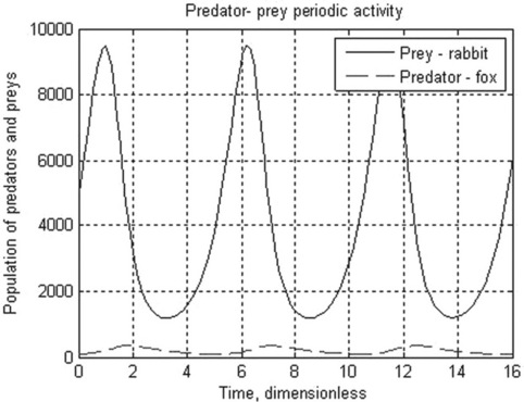
5.1.2.3 Predator–prey Lotka-Volterra model
The Lotka–Volterra is the simplest model for competition between prey, x, and predators, y. With certain simplifications, the model can be represented by the two differential equations:

where k1 and k3 are the growth rate of x (prey, e.g. rabbits) and y (predators, e.g. foxes) species, respectively, and k2 and k4 are coefficients characterizing the interactions between the species.
Problem: Solve the set of ODEs in the time range 0–15 (dimensionless) with initial x = 5000 (rabbits) and y = 100 (foxes). The growth rate constants are: k1 = 2, k2 = 0.01, k3 = 0.8, k4 = 0.0002. Plot the species populations as a function of time, and display the data obtained.
The set of differential equations in the form suitable for ODE solvers
where y1 is x and y2 is y; 0 ≤ t ≤ 5, k1 = 2, k2 = 1.5, k3 = 0.8 and k4 = 0.0002, and initial y1 = 5000 and y2 = 100.
In the absence of a specific recommendation, the ode45 solver should be used. The function file for the set solution is
function t_prey_pred = PredPrey(k1,k2,k3,k4,ts,tf,x0,y0,n)
%To run: > > t_t_prey_pred = PredPrey(2,0.01,0.8,0.0002,0,15,5000,
[t,y] = ode15s(@LotVol,tspan,[x0;y0],[],k1,k2,k3,k4);
plot(t,y(:,1),‘-’,t,y(:,2),‘--’)
ylabel(‘Amount of predators and preys vs time’)
legend(‘Prey –rabbit’,’Predator –fox’)
t_n = linspace(ts,tf,n);% n time points for displaying
y_n = interp1(t,y,t_n,’spline’);% n concentrations for displaying
function dy = LotVol(t,y,k1,k2,k3,k4)
dy = [k1*y(1)-k2*y(1)*y(2);-k3*y(2) + k4*y(1)*y(2)];
The input arguments, k1, k2, k3, k4 and x0 and y0 are, respectively, the same as the k1 k2, k3, k4 and y1 and y2 values at t = 0 in the original set; the tspan is a two-element vector with starting and end t values; and n is the number of points for display. The t_prey_pred output argument is a three-column matrix with the t and population values of prey and predator. Here as in the preceding examples the n rows of t and y values are obtained by the linspace and interp1 commands.
After running this function in the Command Window the following results are displayed and plotted:
> > t_prey_pred = PredPrey(2,0.01,0.8,0.0002,0,16,5000,100,15)
| 0 | 5.0000 | 0.1000 |
| 0.0004 | 7.2701 | 0.1189 |
| 0.0013 | 8.3263 | 0.2799 |
| 0.0022 | 2.5578 | 0.3399 |
| 0.0032 | 1.1982 | 0.2061 |
| 0.0045 | 2.2467 | 0.1102 |
| 0.0062 | 9.4895 | 0.1968 |
| 0.0071 | 3.8686 | 0.3564 |
| 0.0080 | 1.4043 | 0.2659 |
| 0.0092 | 1.4701 | 0.1400 |
| 0.0111 | 8.3298 | 0.1367 |
| 0.0122 | 5.0035 | 0.3521 |
| 0.0131 | 1.5950 | 0.2897 |
| 0.0142 | 1.2852 | 0.1607 |
| 0.0160 | 6.0432 | 0.1060 |
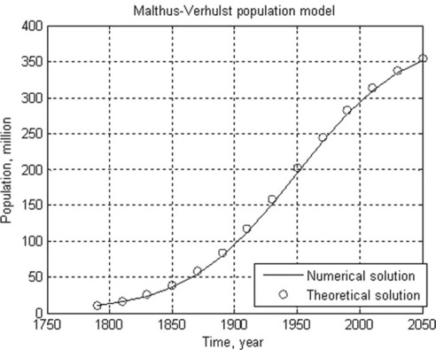
5.1.2.4 Malthus-Verhulst population model
The Malthus–Verhulst ODE is frequently used in population dynamics:
where N is the population size, r is the population growth/decline rate coefficient and K is the maximum population the environment can support. This equation has an analytical solution:
in which C = 1/Nref – 1/K, and Nref is a reference point of the population data.
Problem: Solve numerically the Malthus–Verhulst differential equation with initial N0 = 8.5 million people, and constants K = 395.8 and r = 1.354 (values drawn from USA population statistics). Time is given as a centered and scaled parameter (t - 1890)/62.9 with t = 1790, 1810, …, 2050; calculate N also with the analytical solution equation when Nref = 62.9, at (t - 1890)/62.9 = 0. Plot the numerical and theoretical solution data in the same graph.
The solution is realized in the following steps:
1. The differential equation is solved; for this it should be rewritten in the form suitable for ODE solvers:
The time range is (1790–1890)/62.9 … (2050–1890)/62.9, and initial y0 = 8.5. The ode45 solver is chosen for this equation.
2. The theoretical solution is obtained by the analytical equation at the time values defined in the previous step.
Create for solution the Population function file:
function t_numeric_theoretic = Population(r,K,N0,tspan)
% To run: > > t_numeric_theoretic = Population(1.354,395.8,8.5,[1790:
[t1,y] = ode45(@MaltVerh,t1,N0,[],r,K);
tspan = tspan’; % row to column for including in t_numeric_theoretic
y_theor = K./(1 + K*(1/62.9-1/K)*exp(− r*t1);
t_numeric_theoretic = [tspan,y,y_theor];
plot(tspan,y,tspan,y_theor,’o’)
xlabel(‘Time, year’), ylabel(‘Population, million’)
title(‘Malthus-Verhulst population model’)
legend(‘Numeric solution’,’Theoretical solution’,’Location’,’Best’)
The input arguments for the Population function, r, K and N0, are the same as the r, K and y0; tspan is here a row vector with years given with the colon (:) operator – [1890:20:2050].
The output argument is the t_numeric_theoretic three-column matrix with time in the first column, the population obtained by the ode45 solver in the second and the population calculated by the theoretical expression in the third.
After running this function in the Command Window, the following results are displayed and plotted:
> > t_numeric_theoretic = Population(1.354,395.8,8.5,[1790:20:2050])
| 1.7900 | 0.0085 | 0.0081 |
| 1.8100 | 0.0130 | 0.0124 |
| 1.8300 | 0.0198 | 0.0189 |
| 1.8500 | 0.0298 | 0.0285 |
| 1.8700 | 0.0442 | 0.0425 |
| 1.8900 | 0.0645 | 0.0620 |
| 1.9100 | 0.0916 | 0.0884 |
| 1.9300 | 0.1258 | 0.1219 |
| 1.9500 | 0.1658 | 0.1614 |
| 1.9700 | 0.2086 | 0.2042 |
| 1.9900 | 0.2505 | 0.2463 |
| 2.0100 | 0.2879 | 0.2843 |
| 2.0300 | 0.3186 | 0.3158 |
| 2.0500 | 0.3422 | 0.3401 |
5.2 Solving partial differential equations with the PDE solver
Given the relevance of PDEs in certain biological disciplines, a short introduction to the MATLAB® PDE solver is given here. This solver is designed for the solution of spatially one-dimensional (1D) PDEs and can be used for a single equation or a set that can be presented in the standard form:

where time t is defined in the range t0 (initial) to tf (final) and the coordinate x between x = a and b; m can be 0, 1 or 2 corresponding to slab, cylindrical or spherical symmetry, respectively, the first case representing the elliptical and the other two the parabolic PDE type. Accordingly, the MATLAB® PDE solver is suitable for elliptical or parabolic PDEs only;  is called a tlux term, and
  a source term.
The initial condition for this equation is
and the boundary condition at both points x = a and x = b is

Note that in this equation the same f function is used as previously in the PDE.
In the case of two or more PDEs the c, f, s and q terms in the standard equation can be written as column vectors; in this case element-by-element operations should be applied.
The functions in these equations are subject to certain restrictions which will be explained below. More detailed information is obtainable by typing
or by using MATLAB® Help. The pdepe is the solver command for solution of PDEs.
5.2.1 The steps of PDE solution
Solution of a single PDE goes through the following steps:
1. First, the equation should be presented in the accepted form.
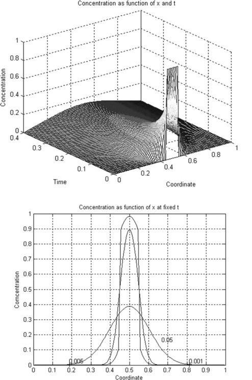
For example, consider the simple diffusion equation for the temporal change of a component concentration:

All variables in this equation are given in dimensionless units, x ranging from 0 to 1, and t from 0 to 0.4. The initial (t = 0) concentration is u = 1 at x between 0.45 and 0.55 and u = 0 elsewhere. The boundary conditions are
The dimensionless diffusion coefficient D is taken as 0.3.
Comparing this equation with the standard form, we obtain:
Thus, the diffusion equation in standard form can be rewritten as:
2. The initial and boundary conditions should be presented in standard form.
To obtain these equations, the following conventions were used:
3. . At this stage the pdepe solver and the functions with the solving PDE, with initial conditions, and boundary conditions should be used. The pdepe solver command has the form
sol = pdepe(m,@pde_function,@pde_ini_cond,@pde_bon_ cond,x_mesh,tspan)
where m is 0, 1 or 2 as above. The pde_function is the name of the function where the solving differential equation should be written; its definition line reads
function [c,f,s] = pdefun(x,t,u,DuDx)
the arguments x, t, u, DuDx, c, f and s being the same x, t, u, ∂u/∂x, c, f and s as in the standard form; the derivative ∂u/∂x in standard expression should be written DuDx. The command pde_ini_cond is the name of the function with the initial condition of the solving equation; its definition line reads
u0 being the vector u(x) value at t = 0. pde_bon_cond is the name of the function with the boundary conditions; its definition line reads
function [pa,qa,pb,qb] = pde_bon_cond(xa,ua,xb,ub,t)
xa = a and xb = b being the boundary points, ua and ub the u values at these points, pa, qa, pb and qb being the same as in the standard form, and representing the p and q values at a and b; x_mesh is a vector of the x-coordinates of the points at which the solution is sought for each time value contained in the tspan; the serial number of each such point and the respective coordinate should be given at the appropriate place; xmesh values should be written in ascending order from a to b; tspan is a vector of the time points as above; the t values should likewise be written in ascending order.
The output argument sol is a 3D array comprising k 2D arrays (see Section 2.2) with i rows and j columns each. Elements in 3D arrays are numbered analogously to those in 2D arrays; for example, sol(1,3,2) denotes a term of the second array located in the first row of the third column, and sol(:,3,1) denotes in the first array all rows of the third column. In the pdepe solver sol(i,j,k) denotes defined uk at the ti time- and xj coordinate points; for example, sol(:,:,1) is an array whose rows contain the u values at all x-coordinates for each of the given times; k = 1 for a single PDE, and k = 1 and 2 for a set of two PDEs.
To solve the diffusion equation of our example, the program written as a function and saved in the file with name mydiffusion is:
function mydiffusion(m,n_x,n_t)
% To run: > > mydiffusion(0,100,100)
xmesh = linspace(0,1, n_x);tspan = linspace(0,0.4, n_t);
sol = pdepe(m,@mypde,@mydif_ic,@mydif_bc,xmesh,tspan);
[X,T] = meshgrid(xmesh,tspan);
xlabel(‘Coordinate’),ylabel(‘Time’), zlabel(‘Concentration’)
title(‘Concentration as function of x and t’)
c = contour(X,u,T,[0.001 0.005 0.05]);
xlabel(‘Coordinate’), ylabel(‘Concentration’)
title(‘Concentration as function of x at constant t’)
function [c,f,s] = mypde(x,t,u,DuDx)
function [pa,qa,pb,qb] = mydif_bc(xa,ua,xb,ub,t)
The mydiffusion function is written without output arguments; its input arguments are: m, as above, and n_x and n_t are the serial numbers of the operative x and t points of the solution. This function contains three subfunctions: mypde comprising the diffusion equation, mydif_ic defining the initial condition and mydif_bc defining the boundary conditions. The x_mesh and tspan vectors are created with two linspace functions in which the n_x and n_t are inputted by the mydiffusion. The numerical results are stored in the sol 3D array, rewritten as a 2D matrix u for subsequent use in the graphical commands. The mesh command is used to generate the 3D mesh plot u(x,t) and the contour and clabel commands – to generate the 2D plot u(x) with the iso-time lines defined in the contour as the vector of the selected t values.
After running this function in the Command Window:
the following two plots are generated (Figure 5.2, p. 156). The clabel command fortuitously superimposes the labels 0.001 and 0.05 on one another and they were separated with the plot editor (see subsection 3.1.3.2) so as not to overburden the program.
In the case of multiple PDEs, the c, f and s functions in the general PDE form and the u0, p and q in the initial and boundary value equations are column vectors.
5.2.2 Application examples
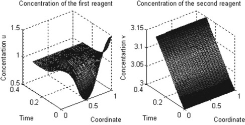
5.2.2.1 Reaction–diffusion two-equation system
For bio-mathematical models, a set of two reaction–diffusion equations is used:
where u and v are concentrations of the participating reagents; all parameters are dimensionless, x varying from 0 to 1 and t from 0 to 0.3.
The level values replaced by the Plot Editor.
The initial conditions are assigned as
and the boundary conditions as
Problem: Solve the set of two PDEs with given initial and boundary conditions and present the changes in the concentrations with time t and along coordinate x.
Rewrite first the set in the standard form
where u1 is u and u2 is v; the m argument is 0 and efficients with x0 and x- 0 are absent.
Note: Element-wise multiplication is used here (see subsection 2.2.2), and thus the left-hand part is apparently the vector 
The initial conditions in the standard form are

and the boundary conditions at x = a and x = b are:
Now write the ReactDiff function file in the form of function without arguments:
xmesh = linspace(0,1,n_x);tspan = linspace(0,0.3,100);
sol = pdepe(m,@ReactDiffPDE,@ReactDiff_ic,@ReactDiff_bc,xmesh,tspan);
[X,T] = meshgrid(xmesh,tspan);
xlabel(‘Coordinate’),ylabel(‘Time’),zlabel(‘Concentration u’)
title(‘Concentration of the first reagent’)
xlabel(‘Coordinate’),ylabel(‘Time’),zlabel(‘Concentartion v’)
title(‘Concentration of the second reagent’)
function [c,f,s] = ReactDiffPDE(x,t,u,DuDx)
s = [1/(1 + u(2)^2);1/(1 + u(1)^2)];
The ReactDiff function is written without output arguments, and its input arguments are: m as above, and n_x and n_t are the numbers of x and t points required. As in the single-PDE example, three sub-functions are involved: the ReactDiffPDE comprising the two reaction–diffusion equations written in the two-row matrices c, f and s, ReactDiff_ic defining the initial conditions in the two-row matrix u0, and mydif_bc defining the conditions at x = a and x = b. The xmesh and tspan vectors are created with two linspace functions. The numerical results are stored in the sol 3D array, rewritten as 2D matrices u and v for subsequent use in the graphical commands. Two subplot commands are used to place two graphs on the same page: surf for generating the 3D surface plots u(x,t) and v(x,t), and axis square for rendering the current axis box square in shape.
After running this function in the Command Window the following plots are generated:
5.2.2.2 Model for the first steps of tumor-related angiogenesis
Tumor-related angiogenesis is an important subject of current oncology research. The first steps of this phenomenon are described by a set of two PDEs:3
where N is the total cell population, n is the concentration of the capillary endothelial cells (ECs), c is that of fibronectin, and d, a, s and r are experimentally determined constants. In dimensionless form these coefficients were obtained as N = 1, d = 0.003, a = 3.8, s = 3 and r = 0.88.
The initial conditions have small alterations along x and are described by the step functions

Problem: Solve the set of PDEs with the given initial and boundary conditions. Plot the solution in two graphs n(x,t) and c(x,t).
First present the PDEs set in standard form:
where u1 and u2 are n and c, respectively; as in the preceding example, the element-wise multiplication yields the vector  .
.
Now present the initial and boundary conditions in standard form:
Here, as earlier, a and b are the boundary points.
To solve the problem, write the tumour function file:4
x = linspace(0,1,xpoints); t = linspace(0,100,tpoints);
sol = pdepe(m,@tumour_pde,@tumour_ic,@tumour_bc,x,t);
n = sol(:,:,1); c = sol(:,:,2);
title(‘Distribution of fibronectin, c(x)’);
xlabel(‘Distance x’); ylabel(‘Time t’);
title(‘Distribution of ECs, n(x)’);
xlabel(‘Distance x’); ylabel(‘Time t’);
function [c,f,s] = tumour_pde(x,t,u,DuDx)
d = 1e-3; a = 3.8;S = 3; r = 0.88; N = 1;
f = [d*DuDx(1) - a*u(1)*DuDx(2);DuDx(2)];
s = [S*r*u(1)*(N - u(1)); S*(u(1)/(u(1) + 1) - u(2))];
function [pa,qa,pb,qb] = tumour_bc(xl,ul,xr,ur,t)
The tumour function is written without input and output arguments; within it, the xmesh and tspan vectors are created with two linspace commands for the selected numbers of x and t points: 81 and 21, respectively; m = 0 as described above. Again, three sub-functions are involved: the tumour_PDE, containing the commands for constants d, a,S, r and N; and two PDEs written in the two-row matrices c, f and s, namely the tumour_ic, defining the initial conditions in the two-row matrix u0, and tumour_bc defining the conditions at x = a and x = b. The numerical results are stored in the 3D sol array, rewritten as the two 2D matrices u and v for subsequent use in the graphical commands. Two subplot commands are used to place two graphs on the same page: the surf commands generate the 3D surface plots u(x,t) and v(x,t), and the axis square commands render the current axis box square in shape.
After running this function in the Command Window
the following plots are generated:

5.3 Questions for self-checking and exercises
1. Which ODE solver is recommended for an ODE, when the class of the problem is unknown in advance: (a) ode23, (b) ode45, (c) ode15s, (d) ode113?
2. For a stiff ODE, which of the following solvers should be tried first: (a) ode15s, (b) ode15i, (c) ode23s, (d) ode23tb?
3. The tspan vector specifying the interval of solution in the ODE solvers should have: (a) at least one value of the starting point of the interval, (b) at least two values –the starting and end points of the interval, (c) several values of the interval, including the starting and end points, or are (d) the two latter answers correct, (e) the answers to (a) and (c) correct?
4. In the pdepe solver a vector xmesh specifies: (a) x and t coordinates to solve PDEs, (b) x coordinates of the points at which a solution is required for every time value, (c) the t coordinates of the points at which a solution is required for every x value?
5. How many and which functions should be written to solve a PDE with the pdepe solver: (a) one function with PDE, (b) two functions, with PDE and with the initial condition, (c) three functions, with PDE, with the initial condition and with the boundary condition?
6. Tumor growth rate is described by the following ODE:
where x is the size of the tumor. The coefficients a and b equal 0.9 month- 1 and 0.7 month- 1 cm- 1, respectively. Solve this equation numerically with the ODE solver in the time interval 0–8 months; initial value x0 = 0.05 cm. Write a function with input and output arguments and save it in a function file. Display the x values obtained at n = 8 equidistant time points, and plot the x,t graph.
7. According to data for the 1918 influenza pandemic, the rate of spread of new infections is described by the equation
where R is the number of new cases per day (called the basis reproductive number); the mean generation time μ = 2.92 days and the variance σ2 = 5.57 days2 are statistical data. Solve this equation numerically with an ODE solver in the time interval 0–15 days with initial R0 = 20. Write a function with input and output arguments and save it in a function file. Display the R values obtained at n = 8 equidistant time points, and plot the R,t graph.
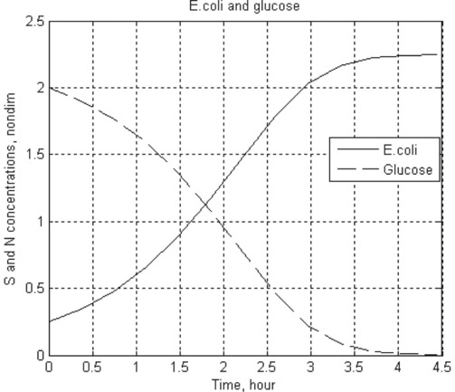
8. Reproduction of the Escherichia coli bacterium on glucose is described by the following set of dimensionless ODEs:
where ![]() is the dimensionless concentration of glucose,
is the dimensionless concentration of glucose, ![]() the bacteria population and
the bacteria population and ![]() is time; S and N are dimensional concentrations in g/L, and t is dimensional time in hours; the reaction rate constant r = 1.35 h- 1, and the constants a = 0.004 g/L and γ = 0.23.
is time; S and N are dimensional concentrations in g/L, and t is dimensional time in hours; the reaction rate constant r = 1.35 h- 1, and the constants a = 0.004 g/L and γ = 0.23.
Solve this set numerically in the time interval 0–6 h at steps of 0.5 h, take initial values ![]() and
and ![]() . For solution use the ode2 3 function. Display the three-column array with dimensional t, S and N values. Plot the
. For solution use the ode2 3 function. Display the three-column array with dimensional t, S and N values. Plot the ![]() and
and ![]() curves.
curves.
9. In a batch reactor two reactions, A → P and A + A → U, take place with rate constants k1 = 2 for the first and k2 = 1 for the second, in arbitrary units. P is the desired product and U an undesired product. These processes are described by the following set of ODEs:
where [A], [P] and [U] are the amounts of species A, P and U, respectively.
Solve these equations numerically in the time interval 0–1 with initial [A]0 = 2 and [P]0 = [U]0 = 0. Plot the [A](t), [P](t) and [U](t) curves.
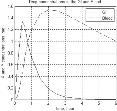
10. In pharmacokinetics the dissolution rates of a drug in the gastrointestinal (GI) tract and in the blood are described by the following set of two stiff equations:

where x and y are the amounts of drug in the GI tract and in the blood, respectively, a and b are the corresponding half-lives of the drug, and D(t) is the dosing function. It is assumed that a drug is taken every 6 hours and dissolves within 30 min. D(t) is described by the following equation
where D is in mg, and ‘floor’ denotes rounding towards minus infinity. The coefficients a and b are 1.38 h- 1 and 0.138 h- 1, respectively.
Solve the set of ODEs numerically with zero initial drug amounts in the GI tract and in the blood. Time values are 0, 0.15, 0.3, 0.6, 0.9, 1, 1.5, 2, 2.5, 3, 4, 5 and 6 hours. Plot the x(t) and y(t) curves.
11. The classical predator–prey model describes the decline in proliferation due to prey crowding.5 The set of equations for this model is
where x and y are populations of prey and predators, the prey survival factor k1 = 1.0019 year- 1, the prey death factor k2 = 1.00224 year- 1, the predator survival factor k3 = 0.999914 year- 1, the predator death factor k4 = 1.0058 year- 1 and the prey crowding factor k5 = 0.101331 year- 1.
Solve these ODEs in the time interval 0–20 years with initial conditions x0 = 2000 and y0 = 2000. Plot the x(t) and y(t) curves, and x versus y in the phase plane graph.
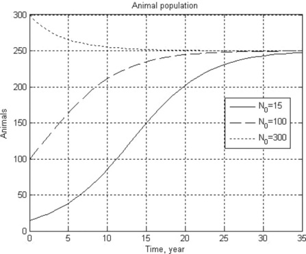
12. An animal population growth rate is described by the differential equation

where N is the animal population, t is time, K is the environmental carrying capacity and r is the growth rate coefficient. For the gray wolf population in one of the American states K = 250 animals and r = 0.21 year- 1.
Solve this equation numerically in the time interval 0–35 years with initial N0 = 15,100 and 300 wolves. Plot all the results in one N(t) graph, and use a constant number of the N-points for all N(t) curves.
13. A bio-fuel (ethanol) is produced from plant tissue by hydrolyzing the cellulose and fermenting the resulting glucose. The process is described by the following equations:6


where [C], [S], [X] and [P] are the concentrations of the cellulose, substrate (glucose), enzyme cells and product (ethanol), respectively;
The constants in these equations are assumed: Et = 1000 mg protein, k = 0.3 mM glucose/(mg protein h), Km = 4 mM, Ki = 0.5 mM, Ks = 0.315 g/L, [P]max = 87.5 g/L, μmax = 0.15 g EtOH/(g cells h), E = 0.249, YX/S = 0.07 and n = 0.36.
Solve the set of ODEs in the time interval 0–10 hours with initial concentrations [C]0 = 125 g/L, [X]0 = 1 g/L and [X]0 = [P]0 = 0. Plot the [C] and [P] concentrations obtained versus time.
14. The diffusion in a biochemical reaction is described by the Brusselator-type PDEs:

where u and v are the species concentrations, and the diffusion coefficient a = 0.02.
Solve this set of PDEs in the time interval 0–10 and coordinate interval 0–1 with the initial conditions

Plot the u and v concentrations obtained as surfaces u(t,x) and v(t,x), taking the azimuth and elevation angles as − 40° and 30°, respectively.
15. The concentration n of a bacterial culture which is diffusing (due to random motion) and reproducing, depending on the nutrient local concentration c, can be described by the following PDEs:
where Dn and Dc are diffusion coefficients,  is the Michaelis-Menten-type reproduction rate, kmax and kn are constants, and k is the bacterial death rate coefficient. It is assumed that Dn = 2, Dc = 1.2, kmax = 2, kn = 1.9, k = 0.8 and α = 0.3.
Solve these PDEs in the time interval 0–1 and the coordinate interval 0–1 with the initial conditions

Plot the surfaces of the n(t,x) and c(t,x) concentrations obtained on the same page, taking the azimuth and elevation angles as 130° and 45°, respectively.
5.4 Answers to selected exercises
3. (d) The two latter answers are correct.
5. (c) Three functions – with PDE, with initial conditions and with boundary conditions
8. > > t_Glucose_Ecoli = Ch4_8(0.004,0.23,1.35,0,4.5,0.25,2)
| 0 | 0.0002 | 0.0080 |
| 0.3704 | 0.0003 | 0.0076 |
| 0.7407 | 0.0004 | 0.0071 |
| 1.1111 | 0.0006 | 0.0064 |
| 1.4815 | 0.0008 | 0.0055 |
| 1.8519 | 0.0011 | 0.0043 |
| 2.2222 | 0.0014 | 0.0031 |
| 2.5926 | 0.0016 | 0.0018 |
| 2.9630 | 0.0019 | 0.0009 |
| 3.3333 | 0.0020 | 0.0004 |
| 3.7037 | 0.0020 | 0.0001 |
| 4.0741 | 0.0021 | 0.0000 |
| 4.4444 | 0.0021 | 0.0000 |
10. > > t_GI_Blood = Ch4_10(1.38,0.138,0,6,0,0)
| 0 | 0 | 0 |
| 0.1500 | 0.5420 | 0.0576 |
| 0.3000 | 0.9826 | 0.2143 |
| 0.4500 | 1.3409 | 0.4493 |
| 0.6000 | 1.2538 | 0.7190 |
| 0.7500 | 1.0191 | 0.9365 |
| 0.9000 | 0.8285 | 1.1058 |
| 1.0000 | 0.7219 | 1.1966 |
| 1.5000 | 0.3630 | 1.4621 |
| 2.0000 | 0.1822 | 1.5386 |
| 2.5000 | 0.0915 | 1.5233 |
| 3.0000 | 0.0460 | 1.4656 |
| 4.0000 | 0.0116 | 1.3083 |
| 5.0000 | 0.0029 | 1.1476 |
| 6.0000 | 0.0007 | 1.0017 |
12. > > Ch4_12(0.21,250,0,35,[15 100 300])

1Notes
The options can be perused in greater detail by typing help odeset in the Command Window.
2Also often referred to as a continuous stirred-tank bioreactor, CSTB.
3Orme, M.E. and Chaplain, M.A.J. (1996) A mathematical model of the first steps of tumor-related angiogenesis: capillary sprout formation and secondary branching. IMA Journal of Mathematics Applied in Medicine & Biology 13: 73–98.
4The tumour function follows the pdex5 example given in MATLAB® demo; to view it, type and enter > > edit pdex5.
5Compare this model with that discussed in subsection 5.1.3.3
6The problem is reproduced from Mosier, N.S. and Ladish, M.R. (2009) Modern Biotechnology. Connecting Innovations in Microbiology and Biochemistry to Engineering Fundamentals. New York: Wiley, p. 136.