
2
Instrumentation
Plant instrumentation constitutes 6–30% of the cost of all purchased equipment for the plant, and thus up to 5% of total project costs for new plants (Peters and Timmerhaus, 1980). A perusal of the instrumentation trade magazines shows what a fiercely competitive market this is. Suppliers are developing a never-ending range of measurement and actuation devices based on new technologies and materials. In order to understand the context of the control schemes and algorithms addressed in this book, one needs a basic appreciation of the devices available.
2.1 Piping and Instrumentation Diagram Notation
The piping and instrumentation diagram is the most important reference document in both the construction and functioning of a processing plant (Davey and Neels, 1991). Not only is it the means of understanding the operation, but its indexing system also allows location of documents pertaining to individual plant items (such as reactors and pumps), the pipework and the measurement and control equipment and philosophy (Figure 2.1).
Figure 2.1 Example of a piping and instrumentation diagram.
Conventions for showing instrumentation vary with company and national standards (e.g. BS 1646 and DIN 28004). Some examples are presented in Figure 2.2. Up until the 1980s, analogue instrumentation data handling was still common, requiring some specific conventions such as in Figure 2.3.
Figure 2.2 Examples of instrumentation symbols.
Figure 2.3 Instrumentation tag bubble notation.
The development of instrumentation that could perform the required operations (such as PID control or square-root extraction) in a purely analogue context became a very sophisticated art, leading to ingenious fluidic (pneumatic) or electronic circuitry. Apart from the high purchase costs, there was a heavy burden of maintenance, so the advent of data-handling systems based on digital computers was warmly welcomed. On economic grounds, most analogue systems were quickly dumped in favour of modern DCS (distributed computer systems), SCADA (supervisory control and data acquisition) and PLCs (programmable logic controllers) (Figure 2.4). Such systems are highly configurable. No longer would the recording of a signal require a dedicated panel-mounted strip or circular chart (frontispiece). All data could be continuously recorded in a historical database, and accessed at will. Alarm limits could be defined for every signal. The control panel along which sociable operators used to stroll, tapping recorders to ensure free pen movement, disappeared, and was replaced by one or more CRT or LCD displays. The art of being an operator changed, and quite a few of the ‘old school’ moved on. In the digital systems, the functional distinctions ‘I’ and ‘R’ in Figure 2.3 have been lost and are omitted from tags.
Figure 2.4 Distributed control system structure illustrating a range of features.
The growth of the digital systems out of the old analogue systems constrained manufacturers (probably needlessly) into a sort of item-per-item replacement. Clearly, this would reduce the shock for existing personnel. The square-root extraction, ratio, control, alarm and trip calculations stayed in functional blocks which could be interconnected just like the old analogue signals. The computer ‘faceplates’ of PID controllers had the recognisable adjustments from the old control room panel. However, beyond the direct replacement of the old functionality, industries realised that they were now in a completely new situation where every measurement and every control actuator could be accessed simultaneously, and there was almost no constraint on the complexity of any calculation. This opened up a whole new world for control engineers to take the concept of ‘advanced process control’ a lot further.
2.2 Plant Signal Ranges and Conversions
One legacy of the analogue era is the handling of measurement and actuator signals in conventional ranges such as
- 4–20 mA;
- 3–15 psig;
- 20–100 kPag.
With new fieldbus devices, instruments can communicate with the computer control system digitally, avoiding the need to convert current or pneumatic signals into the accepted ranges. Nevertheless, much instrumentation is still being designed around the analogue signal range concept, and one has to be aware that any device will anyway have lower and upper saturation limits. On large plants, these analogue signals are handled as close to the associated plant equipment as possible in signal substations. Signal conditioning (such as smoothing) and A/D or D/A (analogue-to-digital or digital-to-analogue) conversion are handled there, so that communication with distributed and centralised computer facilities thereafter occurs on digital buses (e.g. coaxial, fibre-optic or ‘wireless’ transmissions).
A typical signal conversion sequence is given in Figure 2.5. Note that the information flow, starting from the temperature sensor (a), passes through a sequence of calibrations, in this case each involving an intercept and a slope. Each of these is subject to drift and error, so it is only a foolhardy engineer who simply accepts the engineering values presented in the computer display. A nonlinearity arises from the saturation conditions determined by the conventional signal ranges and the A/D and D/A conversion windows. For example, a 20 mA signal (b) might represent an original temperature measurement (a) anywhere above 120 °C. Regarding the 20% offset of the minimum transmission signal values from zero (e.g. 4 mA, 3 psig), this was originally to aid signal loop continuity checking, since the most likely fault would be an open circuit.
Figure 2.5 Typical signal conversion sequence.
For a pneumatically actuated control valve (air-to-open) as suggested here, the intercept and slope (zero and span) are determined by two nuts on the valve stem which position and tension the return spring. It is conceivable that wear or incorrect set-up might result in a 3 psig signal not quite closing the valve, say leaving it 4% open. There is no feedback of this position, so the operator would be unaware that live steam is still in the system, for example. Often the nuts might be set to close the valve at, say, 4 psig, to ensure a really tight shut-off when a 0% (3 psig) open position is requested. These are but some of the pitfalls to be expected, so the engineer would do well to maintain a healthy scepticism regarding the validity of data on the system and should cross-check wherever possible.
2.3 A Special Note on Differential Pressure Cells
The differential pressure (DP) cell is the ubiquitous workhorse of industrial instrumentation, playing a part in the measurement of flow, pressure and level (Figure 2.6). It is a transmitter in the sense that it receives a pressure signal, converts it linearly into the desired signal range (e.g. 4–20 mA, 20–100 kPag) and retransmits it. In cases where it transmits a current signal, it is sometimes referred to as a P/I transducer (pressure/pneumatic-to-current). Flow measurement techniques relying on the creation of a pressure difference (e.g. orifice plates) usually attempt to work with as small a Δp as possible to minimise pumping power. So in this case the DP cell might receive a signal of, say, 0–20 ″WG, and retransmit in the 3–15 psig range. Here one can think of the device as a high-gain amplifier. Conversely, the pressure inside an ammonia synthesis loop (e.g. 150 barg) might be compared with atmospheric pressure, and the Δp retransmitted in the 3–15 psig range.
Figure 2.6 Installed DP cells: (a) electronic and (b) pneumatic (measuring pressure).
DP cells will be installed close to the point of measurement, so there could still be a need to use a completely pneumatic device (as above) for intrinsic safety in the presence of flammable gases. Commercial electrical DP cells are usually provided in explosion-proof housing, so these are likely to be acceptable in hazardous areas as well.
A DP cell might have a very sensitive diaphragm to measure flow or furnace draught (e.g. 20 ″WG), yet all DP cells are supplied in extremely robust steel housing, to allow for the measurement to occur at a high pressure (e.g. flow in an ammonia synthesis loop). In this case, special precautions need to be taken to ensure that the diaphragm is not inadvertently exposed to a high Δp, for example if one of the impulse lines is disconnected from the plant piping.
Figure 2.7 highlights some important considerations of DP cell installation. When it is being attempted to measure small Δp values, as in the use of an orifice plate for flow measurement, a situation where the impulse lines themselves can exert significant and unknown pressure through vapour locks (in the case of liquids) or liquid slugs (in the case of gases and vapours) must be avoided. After all, the cell is seeking to measure the equivalent of only a few inches of water. Even a horizontal connection, if it undulates, becomes subject to the sum of all slugs trapped in the troughs. Thus, for gases and vapours the lines must be arranged to allow clear drainage of any condensate back into the duct, whilst for liquids one seeks a continuity of liquid all the way back into the liquid flow duct. Assuming the liquid duct is above atmospheric pressure, at start-up one loosens the drain screws on the two cell chambers, to allow the liquid to run freely through each chamber and displace any air present. Such an operation of course must take due regard of any excessive Δp that might arise across the diaphragm.
Figure 2.7 DP cell installation for flow measurement.
An equalising valve is normally installed between the HP and LP ports of the cell. This is the means of setting a zero Δp for the purpose of zeroing the cell. With the equalising valve open, the zeroing adjustment is turned until the cell transmits at the threshold of its signal range, namely 4 mA, 3 psig or 20 kPag. Similarly, the span adjustment can be used to effectively set the top end of the scale, for example by matching correctly to a known applied Δp.
Electronic DP cells may use potentiometric, capacitance, piezoelectric, strain gauge, silicon resonance or differential transformer techniques for interpretation of the diaphragm deflection. In the common 4–20 mA type, the device acts as a variable resistance in the current loop, and actually draws its own power from the same loop.
The principle of a pneumatic DP cell is illustrated in Figure 2.8. The diaphragm deflection varies the distance of a flapper from a nozzle, causing a variable back-pressure. This signal cannot be used directly, as additional movement of air out of the nozzle cavity will vary the calibration. Instead, a relay is used to create a balancing pressure by supplying air to an expansion bellows acting on the same flapper. The latter source is able to supply a greater flow of air at a pressure proportional to the nozzle pressure.
Figure 2.8 Principle of a pneumatic DP cell.
2.4 Measurement Instrumentation
An initial division of measurement instruments is into the categories ‘local’ and ‘remote’. A local device needs to be read at its point of installation, and has no means of signal transmission. Typical candidates are thermodials and Bourdon-type pressure gauges. Occasionally, manometers might be used to indicate differential pressures. Up until the 1980s, local measurements were prolific, and important, with operators patrolling the whole plant at hourly intervals, jotting down the readings on a clipboard. Increasingly now the operational picture is built up entirely from electronic information, whether it is updated on graphical mimic diagrams of the plant, or archived for future analysis. It seems that the additional investment in signal transduction, marshalling, conversion and capture is worthwhile in comparison with manual reading, transcription and data entry.
In the processing industries, there are few measurements requiring the high speeds of response often needed in electrical or mechanical systems. Nevertheless, it is important to bear in mind the impact of the response time constant of an instrument considered for each application. For example, a flue gas O2 measurement might output a smoothed version of the actual composition. A brief O2 deficiency might not be seen, but could be enough to start combustion when the uncombusted vapours meet O2 elsewhere in the ducting.
2.4.1 Flow Measurement
2.4.1.1 Flow Measurement Devices Employing Differential Pressure
Bernoulli's equation for incompressible fluids gives
which expresses the conservation of energy in the flow direction (ρ: density; ν: velocity; h: height; g: gravity; p: pressure). For small pressure changes, this is also an adequate representation of gas flows. So between two points in a flow system the changes must balance as follows:
For systems in which some of the energy is used up in overcoming frictional resistance,
Measurements under turbulent conditions show that Δpf is almost proportional to the square of the total flow rate, whether it be flow through ducts, restrictions, plant equipment, particulate beds or free objects moving through fluids. For example, the Darcy equation for pressure loss along a duct is
where L is the duct length and D is the equivalent diameter. There is a minor secondary dependence on the velocity v since the friction factor f′ is generally correlated using the Reynolds number NRe = ρvD/µ. However, as an approximation, frictional pressure losses are usually thought of in terms of a number of kinetic ‘velocity heads’ (one head = v2/2g). For example, the disorderly expansion of a flow with sudden enlargement of a duct incurs a loss of approximately one velocity head, that is Δpf = ρg(v2/2g).
Venturi Meter
As noted above, the flow rate in a duct, or stream velocity passing an object, can be estimated from the pressure drop occurring along a duct section or across the object. Usually these features will cause a net loss of pressure due to friction. However, the venturi flow meter is an attempt to obtain a measurable pressure difference, yet minimise the overall frictional loss. This becomes important in low-pressure systems such as vacuum distillation pipework, furnace draught or flue gas ducting, where the friction loss might compete with the available delivery pressure, alter the density or affect the vapour–liquid equilibrium significantly. It is common to see tapered venturi duct sections in place on the suctions of forced-draught furnace fans, for the purpose of combustion air flow measurement.
Assuming that the velocity profiles at positions 1 and 2 in Figure 2.9 are uniform, and that the flow is frictionless, a general equation for the total mass flow of incompressible and compressible fluids through a venturi tube is
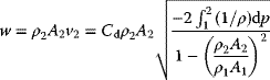
For an ideal gas under adiabatic conditions, this gives
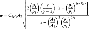
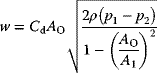
where γ = cp/cv and the pressures are absolute. For p2/p1 close to 1, this reduces to
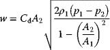
which is also valid for an incompressible fluid. For well-designed venturi meters, the discharge coefficient Cd is found to be around 0.98 for both compressible and incompressible fluids.
Figure 2.9 Venturi flow meter.
Orifice Plate
The orifice plate is the most common flow measurement device employed in the processing industries. There are variations in the installation (e.g. flange tappings versus corner tappings versus upstream/downstream tappings, bevelled edge versus square edge, upstream/downstream free run, etc.), some complying with strict standards.
The principle is the same as for the venturi meter, except that here the precise area of the liquid jet represented by the flow streamlines at the vena contracta in Figure 2.10 is not known. Using instead the area of the orifice itself, one obtains for an incompressible fluid
but now the discharge coefficient is around 0.61 (for high Reynolds numbers), the difference from its value in Equation 2.7 largely compensating for the deviation between A2 and AO.
Figure 2.10 Orifice plate flow meter.
Equation 2.6 suggests that adjustment of Equation 2.8 for compressible flow will depend primarily on γ and the ratios AO/A1 and p2/p1. Indeed, data are available correlating a compressibility factor Y in terms of γ, dO/d1 and Δp/p1 (= 1 − p2/p1).
For a particular fixed installation, users generally rely on the square-root behaviour
where it is seen that
where the compressibility factor Y → 1 for an incompressible fluid.
Calibration of Orifice Plate, Venturi and Similar Flow Meters
In practice, k in Equation 2.9 might be estimated using measured plant displacements. Note that the total volumetric flow rate is obtained as
with the assumption that ρ1 ≈ ρ2, and it is sensible to calibrate in situ to determine the approximately constant k. Indeed, most installations have no compensation for variations in density ρ, with a fixed multiplying constant representing ![]() determined at plant design conditions applied to
determined at plant design conditions applied to ![]() for the form in Equation 2.9.
for the form in Equation 2.9.
Prior to the widespread use of digital computers, the signal for Δp would often arrive at a display panel to be shown on the dial of a simple pressure gauge as in Figure 2.11. The graduations on the dial were simply arranged to extract the square root of the signal, and apply the multiplier K.
Figure 2.11 Square-root extracting flow gauge.
Engineers need to be very wary of this type of mass flow or volumetric flow indication based on a fixed K value. The density of streams on a plant will of course vary with composition, as well as operating pressure and temperature in the case of gases and vapours. The indicated flows must be corrected relative to the calibration condition as in Equations 2.13–2.14 for mass w and volumetric F flows respectively.
It follows for ideal gases that
where M is molecular mass, P is absolute pressure and T is absolute temperature.
A properly calibrated and installed orifice flow meter working at its design conditions can be expected to be accurate to within 2–4% of full span, whilst the accuracy of a venturi meter is around 1% of full span.
Other Flow Measurement Devices Employing Differential Pressure
Figure 2.12 shows three additional flow measurement devices relying on differential pressure. The flow nozzle (a) can be expected to comply with the general equations for venturi or orifice plate meters, and has an accuracy of 2% of span. The Pitot tube (b) has a dynamic port on the tip at which the local pressure will rise by ![]() according to Bernoulli's equation (Equation 2.3), as a result of the velocity being reduced to zero. The static ports just behind the tip provide the offset which allows the local v to be resolved. The device can be simplified using a separate tapping on the pipe wall for the static measurement. The elbow meter (c) is based on the same principle as the Pitot tube, and achieves an accuracy of 5–10% of full span.
according to Bernoulli's equation (Equation 2.3), as a result of the velocity being reduced to zero. The static ports just behind the tip provide the offset which allows the local v to be resolved. The device can be simplified using a separate tapping on the pipe wall for the static measurement. The elbow meter (c) is based on the same principle as the Pitot tube, and achieves an accuracy of 5–10% of full span.
Figure 2.12 Some other flow measurement devices based on differential pressure.
Flow Control Loop Signals
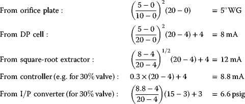
It is useful at this stage to review a detailed piping and instrumentation diagram of a flow control loop, in order to identify the various elements and interconnections arising in the configuration. In Figure 2.13, where only analogue signals are shown, a measurement device requiring square-root extraction is considered, as above. Depending on the audience for an instrument and control scheme representation of this nature, one includes more or less detail. For example, Figure 2.13 might be shown with just a single ‘3FC32’ bubble, and it would generally be understood that the various conversions and the square-root extraction are occurring in this simplified loop. In modern control systems, there are many optional settings for such instrumentation (such as ranges and controller parameters), and this information is usually held in a database, amounting to a number of pages for one loop.
Figure 2.13 Analogue signals around a flow control loop.
It is interesting to follow the sequence of conversions around the control loop in Figure 2.13 for an operating flow of 5 m3 h−1:
2.4.1.2 Other Flow Measurement Devices
As with most industrial instrumentation, there is a plethora of devices based on alternative technologies for flow measurement. The diversity is driven along by manufacturers' attempts to develop new niches based on patents. Indeed, some are well suited to particular environments such as dirty fluids and high-accuracy measurement. Some of these devices are shown in Figure 2.14.
Figure 2.14 Flow measurement devices based on various principles.
Gas mass flow (thermal) devices (g) work on the principle of adding heat to the stream, and detecting its temperature change. In constant-current I mode, the flow rate is inferred from ΔT, and in constant ΔT mode from I. Coriolis meters (h) provide both a flow rate and density. The flow passes through a U-shaped tube which is subjected to a lateral vibration by electromagnets. The flow momentum resists the lateral movement as it enters, and increases that of the other arm of the U as it leaves – causing a phase lag between the two arms which is related to the mass velocity. In turn, the vibration amplitude depends on the stream density.
In Table 2.1, Swearingen (1999, 2001) compares the attributes of selected flow measurement devices. Here ‘variable area’ refers to rotameter-like devices in which an object is displaced (e.g. against gravity or a spring) in order to increase the flow area.
Table 2.1 Comparison of selected flow metering devices (Swearingen, 1999, 2001).
| Attribute | Variable area | Coriolis | Gas mass flow | DP | Turbine | Oval gear | Doppler | Vortex | Magnetic |
| Clean gases | Yes | Yes | Yes | Yes | Yes | — | Yesa | Yes | No |
| Clean liquids | Yes | Yes | — | Yes | Yes | Yes | Yes | Yes | Yes |
| Viscous liquids | Yesa | Yes | — | No | Yesa | Yesb | Yes | Yes | Yes |
| Corrosive liquids | Yes | Yes | — | No | Yes | Yes | Yes | Yes | Yes |
| Accuracy (+/−) | 2–4% S | 0.05–0.15% F | 1.5% S | 2–3% S | 0.25–1% F | 0.1–0.5% F | 2% F | 0.75–1.5% F | 0.5–1% F |
| Repeatability | 0.25% S | 0.05–0.10% F | 0.5% S | 1% S | 0.1% F | 0.1% F | 0.5% F | 0.2% F | 0.2% F |
| Maximum P (psig) | >200 | >900 | >500 | 100 | >5000 | >4000 | Noncontact | 300–400 | 600–800 |
| Maximum T ( |
>250 | >250 | >150 | 122 | >300 | >175 | Noncontact | 400–500 | 250–300 |
| Pressure drop | Medium | Low | Low | Medium | Medium | Medium | Negligible | 15–20 psi | Negligible |
| Turndown ratio | 10 : 1 | 100 : 1 | 50 : 1 | 20 : 1 | 10 : 1 | 25 : 1 | 50 : 1 | 20 : 1 | 20 : 1 |
| Average cost ($) | 200–600 | 2500–5000 | 600–1000 | 500–800 | 600–1000 | 600–1200 | 2000–5000 | 800–2000 | 2000–3000 |
| % S : % of full scale; % F : % of measured flow. | |||||||||
| aWith special calibration. | |||||||||
| b>10 centistokes. | |||||||||
2.4.2 Level Measurement
2.4.2.1 Level Measurement by Differential Pressure
Differential pressure is often used to determine level. Three scenarios are shown in Figure 2.15.
Figure 2.15 Level measurement by DP cell.
Measurements of liquid level for vessels open to atmosphere are obtained from Δp = ρgh, with atmospheric pressure acting on both the liquid surface and the LP port of the DP cell. For enclosed vessels, it is necessary to locate a second sensing point above the liquid surface, to eliminate the effect of any absolute pressure fluctuations. This will involve an extra vertical section of impulse tubing, which introduces the problem of possible condensate collection, for example if the tubing temperature falls below that of the vessel. A serious situation can arise where the actual liquid level is much higher than that indicated. In practice, this problem is dealt with by reversing the DP cell port allocation, and ensuring that the contents of the high leg are known. Typically, the high leg is preloaded with the same liquid as in the vessel. A different, less volatile liquid might be used to avoid re-evaporation as process conditions change, for example glycerine is used in wax crystallisation from MEK.
It is clear that levels obtained from h = Δp/ρg will be dependent on the average density of the liquid. Where this varies much, or froth forms or bubbles are present (as in the boiler ‘swell’ effect), procedures need to make allowance for the possible deviation, or an alternative level measurement technique must be sought.
2.4.2.2 Other Level Measurement Techniques
Figure 2.16 illustrates a few alternative level measurement methods. The bubble tube (a) has an advantage in the case of corrosive liquids or those containing solids or other material that might block impulse lines. Air is bled through the tube to keep the interface at its tip, and this flow must not be so great as to cause an additional frictional pressure drop in the line. Ultrasonic sensors (d) are used for solids hoppers or material with unknown or variable density, for example ice cream. The ball float moving a circular variable resistance (e) is very common, for example in motor vehicle fuel tanks. Radiation (g) and float switches (h) only provide on/off signals as the level crosses the mounting height.
Figure 2.16 Various level measurement techniques.
2.4.3 Pressure Measurement
Figure 2.17 illustrates various pressure measurement devices. As noted in Section 2.3, for low-pressure measurements, collection of liquid in impulse lines must be avoided or compensated for. In all cases shown, the pressure in the duct is being compared with atmospheric pressure, so it is important to qualify the result as a ‘gauge’ pressure, for example 120 kPag or 3.7 barg. A few devices, for example the ionisation gauge for very low absolute pressures, give an absolute pressure. (In this case, a heating element causes ionisation of molecules present, giving a current flow between electrodes which will depend on the number of molecules per unit volume.)
Figure 2.17 Various pressure measurement techniques.
Differential pressure cells (a), or a variation thereof with only one port, are frequently used for pressure measurement. The strain gauge pressure measurement (c) will commonly use an integrated semiconductor incorporating the diaphragm, strain gauge and temperature compensation. The Bourdon tube (e), invented by the French engineer Eugene Bourdon, is the basis of the very common local pressure gauge. The hollow, thin-walled metal crescent flexes as the internal pressure varies. The resultant rotatory motion is captured by a gear system which moves the needle around the dial. Another example of a local indicator is the manometer (f), which may also be used in vacuum applications.
2.4.4 Temperature Measurement
Common devices used for temperature measurement are thermocouples and resistance temperature detectors (RTDs). These are usually encapsulated within a stainless steel rod which can be mounted with or without sheath protection as in Figure 2.18, depending on the application.
Figure 2.18 Sheathed and unsheathed temperature probes.
2.4.4.1 Thermocouple Temperature Measurement
In Figure 2.19a, two wires consisting of different metals are connected at their ends. If the two ends of, say, metal A are at different temperatures, the atomic vibration and electron motion will differ, causing the more energetic hot electrons to tend to drift towards the cooler end. This creates a small potential (emf) across the wire. The same will occur in the metal B wire, but because the metal is different, the characteristic potential differs. As a result, when the two wires are looped as shown, a small current will flow around the loop to balance the net potential. The development of the net potential is known as the Seebeck effect. The emf is almost proportional to the temperature difference. To measure it, the loop is opened and a high-impedance voltage measurement is used (millivoltmeter), to ensure that no further emf changes occur with current flow through the wire resistance. This immediately introduces a problem, because attaching the voltage measurement will create two new dissimilar metal junctions, which will contribute emf depending on their local temperatures. The solution is to make this the reference temperature junction as in Figure 2.19b. A further consideration is that the controlled environment required for the reference temperature will be some distance from the actual plant measurement. Special marked thermocouple cabling of the same metals is used to carry the signal to the reference point, thus avoiding any intermediate dissimilar junctions.
Figure 2.19 Principle of thermocouple temperature measurement.
The common industrial metal alloy combinations used for thermocouples are given in Table 2.2. Type J and E thermocouples give the greatest emf change per unit change in temperature, and are thus suited to more sensitive measurements. Typically, type J varies at 0.05 mV °C−1 whilst type R varies at 0.006 mV °C−1. The variation of emf with the ΔT between the junctions is almost linear for all thermocouples, but not quite. The relationships of ΔT to emf for each type are held in thermocouple tables, which are generally preloaded on plant computer systems, and which are ‘looked up’ with automatic interpolation as the mV signals come in from the plant. Of course, the system needs to know the reference temperature in order to offset the result.
Table 2.2 Common thermocouple metal combinations.
| Type | Metal A | Metal B | Normal range |
| J | Iron | Constantan® | −190 to 760 °C |
| T | Copper | Constantan® | −200 to 371 °C |
| K | Chromel® | Alumel® | −190 to 1260 °C |
| E | Chromel® | Constantan® | −100 to 1260 °C |
| S | 90% platinum + 10% rhodium | Platinum | 0–1482 °C |
| R | 87% platinum + 13% rhodium | Platinum | 0–1482 °C |
2.4.4.2 Metal Resistance Temperature Measurement
As the temperature of a metal increases, the vibration of atoms increasingly impedes the movement of electrons through the material, resulting in a nearly linear increase of resistance with temperature. This is the principle employed in a class of resistance temperature detectors. Platinum and sometimes nickel wire are used for this type of temperature measurement. The fractional change of resistance is around 0.004 °C−1 for platinum and 0.005 °C−1 for nickel, so a resistance bridge with amplifier is used to obtain a usable signal. The resistance is mounted within a protecting tube or sheath, and a small current is used to minimise self-heating under conditions of low dissipation. The device can be set up in a similar way to the thermocouple probe in Figure 2.18, with the additional circuitry for conversion of the resistance to a standard 4–20 mA in a current loop mounted in the cap. For smaller temperature ranges, a linear or quadratic fit is adequate for interpretation of the temperature.
2.4.4.3 Temperature Measurements Using Other Principles
In Figure 2.20, some examples of alternative temperature measurements are given. The thermodial (a), based on a bimetallic spiral in which strips of two dissimilar metals are fastened together, is the very common local measurement seen on plants. As the temperature rises, the two metals expand differently, imparting a turning moment in the spiral. One end of the spiral is fastened to the thermowell wall, whilst the free end rotates the needle on the dial. Liquid temperature indicators, such as mercury or alcohol thermometers, are well known, and can be arranged to impart mechanical movement for indicator dials, or for electrical signals, as in (b). The pressure exerted by a fixed volume of gas can similarly be interpreted as a temperature, for example by the ideal gas law, whereas that exerted by a vapour in equilibrium with its liquid could be used to infer its temperature from a known relationship such as the Antoine equation (c).
Figure 2.20 Temperature measurement using various principles.
The thermistor (d) is made from semiconductor material which has a low electrical conductivity compared with metals, because electrons are more tightly bound to the molecules. As the temperature increases, the molecules vibrate more, imparting energy to the electrons and thus increasing their ability to escape and move through the material. Thus, unlike metals, the apparent resistance decreases as temperature increases. A table or graph is required to infer the temperature from the resistance. Other solid-state devices such as transistors or Zener diodes (e) can be doped so as to give significantly varying voltage as temperature changes. Finally, one notes that any body radiates at a frequency dependent on its temperature, so that optical techniques such as infrared sensors and optical pyrometers can be used to infer temperature. For example, a pyrometer ‘gun’ might be used to sight on individual furnace tubes to determine hot spots.
2.4.5 Composition Measurement
Even in the laboratory, the measurement of composition is based on indirect techniques such as flame ionisation, light transmission or polarisation. On a chemical plant, one usually seeks a simpler indirect measure on the composition which is more robust and does not require the controlled environment and sophisticated calibration inherent in accurate laboratory measurements. Thus, gas density might be used to infer the average molecule size in a hydrocarbon vapour, or liquid density used to determine dissolved sugar (brix), alcohol or HCl. Other indirect techniques might use pH or conductivity. In distillation, where mixtures are binary, or at least have characteristic distributions, a temperature measurement might be used, possibly with a correction for pressure (e.g. Figure 4.23). Other ‘composition’-type measurements required include Kappa value, turbidity, viscosity, knock, octane, flue O2, and heating value. Manufacturers have developed a range of ingenious devices to provide online indications of most of these properties. Only occasionally is an online gas or liquid chromatograph installed. Such an installation tends to be very expensive, and of course can only provide an intermittent measurement update following the injection and purge cycles. A remarkable achievement of the old analogue period was Foxboro's intrinsically safe, plant-mounted process gas chromatograph, powered and programmed pneumatically, with a steam-heated oven, and with eluted gases identified by pressure-drop variations across an orifice (Annino et al., 1976).
Figure 2.21 shows the H+ sensing electrode and reference electrode for pH measurement. These are usually housed within one probe, which also has a sensor for temperature compensation. Note that the nonlinear relationship of pH = −log10([H+]) to the molar concentration of H+ ions [gmol L−1] is a recognised nonlinear control problem.
Figure 2.21 Composite pH probe with both electrodes in one housing.
2.5 Current-to-Pneumatic Transducer
Current-to-pneumatic (I/P) converters are very common industrially. Though some control actuators are electrically driven, most still rely on transmitted instrument air for their motive power. Apart from anything else, air signals are intrinsically safe in the presence of flammable materials. At some stage in the transmission of an output signal from the controller, a conversion must be made to a pneumatic range (3–15 psig or 20–100 kPag). Typically, this conversion is from current to pneumatic, which is illustrated in Figure 2.22.
Figure 2.22 Current-to-pneumatic converter.
The similarity to Figure 2.8 for the pneumatic DP cell is obvious. Again, a relay is used to equate a high-flow output signal to the more sensitive nozzle pressure. Typically, one does not wish to upset the pressure balance around the nozzle whilst a control-valve diaphragm is being inflated.
2.6 Final Control Elements (Actuators)
Most of the final control elements in the processing industries are valves used to regulate the motion of fluids. The focus in this section is on remotely operated valves, but at the outset one notes that there will be many manually operated valves on a plant for less frequent use, as in the common ‘double-block and bypass’ arrangement in Figure 2.23. Control valves sometimes need maintenance, so that they are often located in accessible spots near floor level, to allow disconnection and removal. A means must be provided to prevent residual process fluids from escaping through the vacancy – that is the purpose of manual block valves. Quite often, with communication to an operator at the location, the process can continue to function temporarily with occasional manual adjustments of the bypass valve. A quite undesirable practice is sometimes seen where debottlenecking of a process has led to bypass valves being left partially open in normal operation, just to increase throughput. In addition to the three manual valves involved, two manual bleed cocks will sometimes be provided in liquid systems not only to empty the closed-off sections in a controlled way, but also to avoid trapping of liquid which on thermal expansion might rupture the pipework.
Figure 2.23 Double block and bypass.
2.6.1 Valves
2.6.1.1 Pneumatically Operated Globe Control Valve
The globe control valve (Figure 2.24) is the most common device used for precise flow regulation, and the simple and safe source of motive power for this valve is usually the instrument air system. Figure 2.25 illustrates the workings of an air-to-open globe control valve with positioner. Unlike domestic taps, note that the flow normally approaches from the stem side of the valve plug. An adjustable stuffing box with a gland prevents leakage to the outside.
Figure 2.24 Air-to-open globe control valves without (a) and with (b) a positioner.
Figure 2.25 Air-to-open globe control valve with positioner.
Most control valves can be switched between air-to-open and air-to-close service by simple mechanical adjustments as indicated in Figure 2.26. Bearing in mind that the most likely disaster would be loss of instrument air pressure, or breakage of the pneumatic signal line, the air-to-open (AO) is taken as fail-closed (FC) and the air-to-close (AC) is taken as fail-open (FO). In control scheme design, it is important to make this specification to ensure as orderly a shutdown as possible in the event of disaster, for example furnace fuel supplies will typically be fail closed. For motor-operated valves, or electrical solenoid valves, the fail situation would correspond to loss of the electrical power or signal.
Figure 2.26 Valve air-to-open and air-to-close arrangements with adjustments.
In Figure 2.26, a typical range adjustment provision is shown. A collar allows variation of the stem length, whilst one or two nuts may vary the position and tension on the return spring. It is important to check these adjustments, so that the actual motion of the stem between 0% open and 100% open corresponds as well as possible to the instrument signal range, say 3 and 15 psig (or 15 and 3 psig for an air-to-close valve). A point of caution is that valve signals are occasionally reported as ‘% closed’, so it is wise to qualify the units of measurement as either ‘% open’ or ‘% closed’ when valve position is being discussed.
In Figure 2.27, the arrangement inside a globe control valve with cage and plug is illustrated. The arriving fluid passes through the holes in the cage, around its full circumference. The plug passes up and down within the cage, with the various holes cut into the plug's cylindrical surface overlapping in a predetermined way with the holes in the cage. The fluid passes through this overlap into the hollow interior of the plug, and thus moves downward and out of the valve. It is the way in which the overlap area varies with stem movement that determines the characteristic of the valve, which will be discussed shortly. Whereas the perforated part of the plug passes through a hole in the seat, a protruding edge higher up on the plug provides the means for a tight seal against the seat when the valve is closed.
Figure 2.27 Globe valve showing flow through cage and plug.
2.6.1.2 Valve Characteristics
Any valve, whether manual, automatic, globe or butterfly, has a characteristic. This is a plot of the fraction of the maximum flow achieved whilst the valve ‘position’ is varied from 0 to 100% open, with a constant pressure difference across the valve. The position will be based on either linear stem movement or rotation.
For most process control applications, the linear characteristic would appear to be more suitable, whilst a quick-opening valve might be useful in pressure relief. This characteristic determined under constant valve pressure drop, ΔPV, is called the inherent characteristic. In practice, the actual flow achieved is also dependent on other frictional pressure losses in the remainder of the line flow route including equipment, ΔPL. These will increase as the flow rate increases, and if the overall driving pressure difference ΔPT = ΔPV + ΔPL is fixed, it must mean that the ΔPV available across the valve decreases. The effect is to distort the operating characteristic as in Figure 2.28, which is called the installed characteristic (Figure 2.29).
Figure 2.28 Valve inherent characteristics.
Figure 2.29 Valve installed characteristics.
When the valve is shut, the maximum possible pressure is exerted across the valve, and this reduces as it opens. For lines with large resistances, such as a long hosepipe, this is quite noticeable, as the water first rushes out, and then drops to a lower rate as the available ΔPT becomes distributed elsewhere. Depending on the resistance of the remaining equipment in the line, and the ΔPT available, notice that it should be possible to choose an equal-percentage valve (e.g. α = 30 in Figure 2.28) which restores the f(x) behaviour to approximate linearity. Such a valve would of course be designed to reveal flow area at a greater rate per % opening as it opens further, for example with plug slots broadening towards the bottom.
2.6.1.3 Valve CV and KV
Incompressible Fluids
For incompressible fluids, the volumetric and mass flows through a valve are determined by Equations 2.17 and 2.18, which follow from the orifice equation (Equation 2.11), with the characteristic scaling f(x) for valve opening.
The coefficient ![]() is usually quoted as a numerical value without units, but its units are implied by the following definition:
is usually quoted as a numerical value without units, but its units are implied by the following definition:
This follows because water has a specific gravity of 1 at 60 °F. The effective units are
and for the more general form involving ρ, any units may be used based on
There is an equivalent ‘flow factor’ KV based on SI units, either in m3 h−1 or l min−1:
So
Manufacturers give their valve sizes in terms of CV of KV.
Compressible Fluids
From Equations 2.9 and 2.10 for an orifice of area AO in a duct of area A1, one has
The passage of fluid through the valve restriction behaves in the same way, except that only a fraction f(x) of the fully open area AO is available. Manufacturers (e.g. Fisher Controls International LLC, 2005; Smith and Corripio, 1997) have developed correlations and charts for two corrections, namely a ‘piping geometry factor’ FP and the compressibility factor (‘expansion factor’) Y. These are applied in the form
The expansion factor Y depends on γ = cp/cv, p2/p1 and (p2/p1)CRIT, the critical absolute pressure ratio above which flow becomes independent of p2 (0.53 for air).
2.6.1.4 Specification of Valves for Installed Performance
The dependence of valve performance on other line resistances has been mentioned in Section 2.6.1.2. The flow resistance imposed by a valve has to be ‘significant’ compared with the line resistance, for the whole of the range 0–100% open, otherwise there may be no flow variation as the valve position changes.
In the example shown in Figure 2.30, one notes that a fixed total pressure difference is available to drive the process liquid through line section AB:
This will be absorbed in the line pressure loss ΔpL, dependent on the geometry of the piping and process equipment, and the flow rate, as well as the valve pressure drop, ΔpV, dependent on the valve CV, inherent characteristic f(x) and flow rate (Figure 2.31).
The discussion in Section 2.4.1.1 led to the approximation of frictional pressure losses as a number of kinetic ‘velocity heads’, ρν2/2, which we can re-express as some multiple of density times the square of the total volumetric flow rate.
Though adequate, this is not strictly true, as seen in the Darcy equation (Equation 2.4), where the friction factor f′ would have a secondary dependence on F. For liquid passing through a control valve, Equation 2.17 gives
where kV = 1/k2 for the k in Equation 2.17, or 0.12 US gallon lb−1/![]() according to Equation 2.19. Then Equation 2.24 can be rewritten as
according to Equation 2.19. Then Equation 2.24 can be rewritten as
The situation ![]() could arise where too large a valve CV has been specified, bearing in mind that
could arise where too large a valve CV has been specified, bearing in mind that ![]() . Clearly there would only be a significant change of flow as the valve starts to open (low x giving low f(x)). On the other hand, too large a kV (small CV) would impede flow unnecessarily, giving high energy costs. Various ‘rules of thumb’ have been proposed to preserve a balance between these two resistances, as in Table 2.3.
. Clearly there would only be a significant change of flow as the valve starts to open (low x giving low f(x)). On the other hand, too large a kV (small CV) would impede flow unnecessarily, giving high energy costs. Various ‘rules of thumb’ have been proposed to preserve a balance between these two resistances, as in Table 2.3.
Figure 2.30 Valve to be specified for LC2 on line section AB.
Figure 2.31 Pressure loss contributions for line and valve.
Table 2.3 Examples of valve sizing rules of thumb.
2.6.1.5 Control Valve Hysteresis
Generally, when a control system commands a valve to go to a particular position, there is no feedback evidence of what position is actually achieved, that is the valve operates in open loop. Because of their mechanical linkages and friction, valves are relatively unreliable in this respect. Note at the outset that only the signal sent to the valve is known. In practice, if one varies this signal from 0 to 100% open, and then back to 0% open, the true valve stem position follows as in Figure 2.32.
Figure 2.32 Control valve hysteresis.
The hysteresis behaviour of control valves will arise to some extent from play in the linkages, but one expects that it is largely a result of ‘slip-stick’ friction in the valve stem movement through a tight stuffing box. In Figure 2.32, when the upstroke starts, the signal to the valve increases to 20% open before any stem movement occurs. Effectively, the upward force applied to the stem has increased to 20% of range, before the static friction is overcome and the stem ‘gives’. This excess force has to stay in place for the entire upstroke travel, allowing the stem to move with each incremental signal increase thereafter. As might be expected, the true valve position might never reach 100% open. When the valve signal is reversed, to go downwards from 100% open, the excess force must first be removed, and a similar excess force applied in the reverse direction before the ‘stick’ friction is overcome, and the stem begins to ‘slip’ in the reverse direction.
The misleading aspect of this phenomenon is that one usually obtains system ‘gains’, for example flow per % open, using big valve adjustments. The actual gain experienced by a controller will depend on the size of its adjustment cycles, and these will usually be smaller as in the Figure 2.32 example, giving much smaller effective gains, and often no valve movement at all! The phenomenon is variable and nonlinear, and bound to cause problems in control loops which rely on reasonably linear behaviour. de Vaal, Eggberry and Jones (2006) used phase-plane plots to detect hysteresis in plant control (Figure 2.33).
Figure 2.33 Typical phase-plane plot revealing valve hysteresis.
Industrially, the problem of slip-stick friction in valves is reduced using a valve positioner, as in Figures 2.24 and 2.25. Here the signal transmitted to the valve becomes a position setpoint, and a mechanical controller mounted on the valve compares this value with the actual stem position, obtained using a mechanical link. The local control loop has access to its own air supply, and it applies more or less of this air to the valve diaphragm to bring the feedback position to the setpoint position.
2.6.1.6 Various Flow Control Devices
A great variety of flow control devices exists, suited to different applications. Some are discrete in the sense that they only use two positions, some are designed for accurate regulation and some are designed to handle fluids containing solid particles. In Figure 2.34, the weir and diaphragm valve can be used for particulate-bearing flows, because it is able to flush itself clear. Likewise, the dart plug valve is typically used to control the flow of slurries through flotation cells. Gate or ball valves can be arranged to leave the entire pipe flow area clear, and are thus suited to special cleaning requirements such as the passage of a ‘pig’. Louvres and baffles would be suited to low-pressure systems such as furnace ducting.
Figure 2.34 Various flow control devices.
2.6.2 Some Other Types of Control Actuators
Having considered the major process control requirement of actuators for flow regulation, it is worthwhile before proceeding to mention a few other actuator devices that could play a part in control schemes. Fans, pumps, compressors, electrical heaters, solenoid-driven actuators and electrical shut-off valves normally only have two states – on and off. There are, however, a few electrically driven devices offering scope for intermediate settings. These include thyristor power supplies, variable-speed drives and stepper motors. Hydraulic actuators are not that common in the processing industries. Though mostly discrete in nature, hydraulic devices also exist for intermediate positioning.
2.7 Controllers
The centrifugal governor, developed by James Watt and Matthew Boulton in 1788, was one of the earliest control devices (Figure 2.35). The same principle is still in use for setting the speed of steam-powered turbine drives.
Figure 2.35 Early control devices.
Until the 1980s, panel-mounted analogue controllers similar to Figure 2.36 were common. Sometimes these were integrated within a circular or strip chart recorder. This is the SISO controller which could service a single control loop. With the conversion to computer-based systems, the same concepts and terminology have been retained. The same functions are carried out by programs which run on PLCs or distributed computer cards, and these can continue to function independently if part of the system is damaged. When the operator views a controller on the control room displays of a DCS or SCADA system, it is represented in analogous format. On the conversion of plants to the much cheaper computer-based systems, the control loops were replaced on a one-for-one basis. The many tasks requiring this type of control are referred to as the ‘base layer’ control system, and it will be seen later that the modern advanced control algorithms facilitated by computers tend to communicate with the plant through this layer.
Figure 2.36 Typical panel-mounted analogue controller.
The loop controller has a switch to select either AUTO or MANUAL operation. In the MANUAL mode, it is possible to adjust the control action output directly, using the ‘manual loading station’ at the bottom of the controller in Figure 2.36. In AUTO mode, the device makes use of its internal computation to set a suitable control action output which will bring the feedback signal to the setpoint value.
The other switch on the controller allows selection of LOCAL or REMOTE. In LOCAL mode, the setpoint can be adjusted directly by the operator. In REMOTE mode, this is no longer possible, because the setpoint is manipulated from elsewhere. This could be in a cascade format from a similar SISO controller, or possibly from an ‘advanced’ control algorithm based on several PVs and manipulating several MVs.
The original analogue controllers were used in one of the three control modes: proportional (P), proportional–integral (PI) and proportional–integral–derivative (PID). Rather more features are possible today in the computer equivalent controller. For the analogue devices, one accessed the back of the cabinet to adjust the proportional gain, integral time constant or derivative time constant. These can of course be set remotely in the computer devices.
For computer-based controllers, one usually works in engineering units (e.g. % open, °C, tph, barg), a change from the fractions of standard instrument ranges of the past. The important thing to note with the SISO controller is that it has three different signals. Two of these signals refer to the same variable and will have the same units of measurement, namely the controlled variable feedback and its setpoint. The third signal leg that must attach to the controller bubble on a P&I diagram is the control action, which refers to a different variable and is nearly always in different units. In this sense, the controller can be viewed as a ‘translator’, for example ‘At what [% open] must this valve be set to bring the temperature to 30 [°C]?’ So the algorithm inside the device must iteratively solve an implicit problem, and translate from the ‘language’ of the input to the ‘language’ of the output.
2.8 Relays, Trips and Interlocks
The on/off signals emanating from a control system cannot in general power plant equipment. These are passed to relays designed to close or open circuits carrying the required power. Such a relay typically uses an electromagnet to open and/or close contacts. Such relays were also found useful for ‘latching’ circuits as in the electrical motor start (NO - normally open) and stop (NC - normally closed) button circuit shown in Figure 2.37. The functioning of this latching circuit, involving several digital 0/1 states, can be described in Boolean algebra as a series of interdependent events X and non-events ![]() :
:
| G | GO pushbutton pressed and released |
| S | STOP pushbutton pressed and released |
| C | coil energised closing both relay switches |
| M | motor receives power |
Although the emphasis of this text is on the continuous algorithms which smoothly vary plant parameters, one has to be aware of the network of discrete overrides, interlocks and trips which become superimposed on such algorithms in practice. These generally aim to avoid dangerous or destructive situations from developing; for example, if the tank level exceeds its high limit, switch off the pump. In the past, these protective systems made use of electromagnetic relays as in Figure 2.37. Nowadays, the discrete decision system is programmed directly on the plant computers. Although Boolean or ‘expert system’ forms may be used, ladder diagrams based on the original alternating current relay systems are still widely used to represent the sequence of events and the hardware involved. The equivalent of the circuit in Figure 2.37 then becomes the simple ladder in Figure 2.38. For larger systems, many more rungs can be added to the ladder, forming a clear record of the interrelationship of events. Additional symbols exist for normally open and normally closed limit switches for pressure, temperature, level and position, as well as for timing delays. One way used to ‘trip’ an air-to-open control valve into its shut position is to vent the air signal at the valve by energising a solenoid valve.
Figure 2.37 Latching circuit for motor power.
Figure 2.38 Ladder diagram for discrete logic of circuit in Figure 2.37.
2.9 Instrument Reliability
An important step in the design of new plants, or plant modifications, is the operability study as described by Lawley (1974). This aims to detect problems that could arise from unusual plant operation, for example higher flows or temperatures than expected. These may be resolved by plant equipment changes, but very often lead to the addition of further instrumentation, as well as control and interlocking systems for monitoring and protection. It is not surprising then that when the hazard analysis is performed, the degree of risk becomes highly dependent on instrument reliability. It is useful then to consider some typical failure rates for standard instrumentation (Tables 2.4 and 2.5). Such data might more realistically be estimated simply from experience on the processing plant of interest. Moreover, one notes that most ‘controllers’ are nowadays computer-based, giving failure rates much lower than 0.29 pa on typical high-integrity systems. The intention now is to use these standard component failure rates to estimate the overall probability of failure of a system constructed from these components.
Table 2.4 Typical failure rates for processing plant instruments from Lees (2001).
| Instrument | Failure (faults per year) |
| Control valve | 0.60 |
| Pressure measurement | 1.41 |
| Flow measurement (fluids) | 1.14 |
| Level measurement (liquids) | 1.70 |
| Thermocouple temperature measurement | 0.52 |
| Controller (analogue) | 0.29 |
| Pressure switch | 0.34 |
| pH meter | 5.88 |
| Gas–liquid chromatograph | 30.6 |
| Impulse lines | 0.77 |
Table 2.5 Causes of analogue control loop failure from Lees (2001).
| Element in loop | Faults (%) |
| Sensing/sampling | 21 |
| Transmitter | 20 |
| Transmission | 10 |
| Receiver (e.g. indicators and recorders) | 18 |
| Controller (analogue) | 7 |
| Control valve | 7 |
| Others | 17 |
Figure 2.39 represents a fired boiler control scheme in which two protective trip systems activate as excessive pressure levels are reached. When the high limit PA is reached, fuel to the furnace is cut off, and when the next high limit PB (PB > PA) is reached, steam is vented directly from the drum. What one is concerned about in a hazard analysis is the possibility of the pressure rise occurring and going completely unchecked, based on a few possible failures, which might be defined as follows:
| V1 | fuel valve (open) |
| FT1 | fuel flow measurement (too low) |
| FC1 | analogue fuel flow controller (valve output too high) |
| PC2 | analogue pressure controller (output sp to FC1 too high) |
| PT2 | pressure measurement (too low) |
| PAH2A | first pressure trip (does not activate) |
| PAH2B | second pressure trip (does not activate) |
| Fhigh | fuel flow higher than setpoint |
| Fsphigh | fuel flow setpoint too high |
| Phigh | occurrence of excessive pressure in drum |
| Pexplode | final high-pressure failure |
Figure 2.39 Boiler pressure control with two trip levels.
The various events can be related by Boolean logic as follows:
A fault tree diagram represents this sequence as in Figure 2.40. A few useful results when evaluating fault trees include
Figure 2.40 Fault tree for boiler pressure control with two trip levels.
De Morgan's theorem:
Quite often evaluation of the Boolean expression for the main event reveals a simple underlying cause, for example a fire which both overheats a vessel and destroys shutdown trip cabling. It turns out that the same expressions can be used to determine the probability of an event occurring. Here one has to think of ‘A’ as the probability that this state will exist at any instant in time.
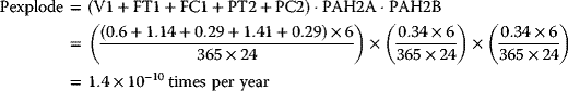
The available data such as in Table 2.4 are unlikely to have such detail as the direction of failure (shown in parentheses above). However, if one uses the frequency as stated, one will certainly arrive at a probability representing the worst-case scenario. Take for example the equivalent probability for V1. According to Table 2.4, a control valve can be expected to fail 0.6 times per year. One needs to think of an average time for detection and rectification of such a situation – say 6 h. So in 1 year, a single valve will spend 3.6 h in its failure state, representing a time fraction of 0.0004. One notes that the probability of this event not occurring ![]() , and that the probability that both V1 and V2 will be in a failed state simultaneously is V1·V2 = 16 × 10−8, or that either will be in a failed state is V1 + V2 = 0.0008, and so on. Arbitrarily taking a detection and rectification time of 6 h for all of the events in Table 2.4, the Boolean expression (Equation 2.34) determined above gives the frequency:
, and that the probability that both V1 and V2 will be in a failed state simultaneously is V1·V2 = 16 × 10−8, or that either will be in a failed state is V1 + V2 = 0.0008, and so on. Arbitrarily taking a detection and rectification time of 6 h for all of the events in Table 2.4, the Boolean expression (Equation 2.34) determined above gives the frequency:
Of course, one is unlikely to derive a single final equation like Equation 2.48 for large systems. The computational algorithm used will more likely be built on a sequence of intermediate evaluations as in Equations 2.30–2.33.
An equivalent way of doing this calculation is to simulate the underlying phenomena using a Monte Carlo technique. Consider the vector of component status Boolean variables
to be randomly drawn from a ‘top-hat’ probability density function as in Figure 2.41 according to the rule that a value of 1 results for the sample x lying in the range 0–probability of state, and 0 otherwise. For example, if the sample drawn for V1 lies between 0 and 0.0004, then the result is 1, and 0 otherwise. Clearly the frequency of a ‘TRUE’ result will match each variable's individual probability. Each fresh ‘realisation’ of the Boolean vector is inserted into Equations 2.30–2.33 to get the state of Pexplode (0 or 1) for this realisation. As more realisations are used, the frequency of a TRUE result (i.e. 1) for Pexplode must approach 1.4 × 10⁻¹⁰ times per year.
Figure 2.41 ‘Top-hat’ probability density function.
This idea has been taken further by Hauptmanns and Yllera (1983) to describe a particular situation where either the failure of a component item is not detected or rectification cannot be effected. It has been noted that the distribution of times of failure of such items follows an exponentially decreasing function as in Figure 2.42. This can be understood in the sense that 100 equal items all starting out at time zero will have an ever-decreasing failure time density as items are eliminated. For human beings, the mean time to failure is around 75 years!
Figure 2.42 Unrecoverable failure time distribution for an item type ‘i’.
Samples of failure time are drawn from a distribution like Figure 2.42 for each item i. It is noted that this distribution is easily simulated by drawing a sample x from a unit top-hat distribution as in Figure 2.41, and subjecting the result to the conversion
For the valve V1 in Figure 2.39, Table 2.4 gives a failure frequency of 0.6 pa, suggesting a mean time to failure TV1 = 1/0.6 = 1.7 years.
If the failure time t thus obtained is less than some defined mission time TM, then the failure of that component is considered to have occurred, and the corresponding Boolean value is set to 1, else it is set to 0. In this way, a single realisation of the component status Boolean vector is evaluated as before, and used to evaluate the overall failure status of interest. Repeated sample realisations of the component vector will give further values of the overall failure status (0 or 1), from which the probability of failure by a chosen time TM may be evaluated. Repeating this at a series of mission times TM allows the cumulative probability F(TM) of the failure of interest within the mission time TM to be evaluated. As shown in Figure 2.43, this can be differentiated to get the probability density function f(TM) of the overall failure of interest with time.
Figure 2.43 Cumulative probability and probability density of overall failure with mission time.
References
- Annino, R., Curren, J., Kalinowiski, R., Karas, E., Lindquist, R. and Prescott R. (1976) Totally pneumatic gas chromatographic process stream analyzer. Journal of Chromatography, 126, 301–314.
- Davey, W.L.E. and Neels, J. (1991) The engineering of complex projects. 6th National Meeting of the South African Institution of Chemical Engineers, Durban, August 7–9, 1991.
- de Vaal, P.L., Eggberry, I. and Jones, M. (2006) Methods to detect causes of control loop oscillations. SACEC 2006: Engineering Africa in the 21st Century, South African Institution of Chemical Engineers, p. 12.
- Fisher Controls International LLC (2005) Control Valve Handbook, 4th edn, Fisher/Emerson Process Management.
- Hauptmanns, U. and Yllera, J. (1983) Fault-tree evaluation by Monte-Carlo simulation. Chemical Engineer, 90, 91–103.
- Lawley, G. (1974) Operability studies and hazard analysis. Chemical Engineering Progress, 70, 45–55.
- Lees, F.P. (2001) Loss Prevention in the Process Industries, 2nd edn (revised), vol. 1, Butterworth-Heinemann.
- Peters, M.S. and Timmerhaus, K.D. (1980) Plant Design and Economics for Chemical Engineers, McGraw-Hill.
- Smith, C.A. and Corripio, A.B. (1997) Principles and Practice of Automatic Process Control, 2nd edn, John Wiley & Sons, Inc., p. 204.
- Swearingen, C. (1999) Selecting the right flowmeter – part 1. Chemical Engineering Magazine, July 1999.
- Swearingen, C. (2001) Selecting the right flowmeter – part 2. Chemical Engineering Magazine, January 2001.