
5
Control Strategy Design for Processing Plants
The piping and instrumentation diagram (Section 2.1) is the key document describing a processing plant, around which the rest of the design revolves. In the design and construction phases, it must be kept up-to-date, and in computerised documentation systems it will be found to link automatically to virtually every other design document. So at an early stage, it becomes necessary to specify the plant instrumentation scheme and control philosophy. The objective of the control engineer is initially that the plant ‘should be able to take care of itself’ under most circumstances. Once that objective is reached, he or she will seek to get the plant to ‘take care of itself optimally’. This rests on the field of advanced process control, arising from the common use of digital computers. As industries have improved their safety, efficiency and product specification compliance through advanced approaches, so too have their competitors been obliged to develop advanced control capacity, in order to remain competitive.
In modern processing plants, the processing scheme itself is becoming more complex, owing to flow scheme optimisations such as ‘pinch’ technology which seeks to minimise energy demands or waste streams. These developments lead to a lot of interactions across the plant, for example heat recovery interchange after a reactor. It is understandable that this complicates plant control – how does one get a stream up to its reaction temperature when it requires the exothermic reaction heat to get there? At one time just a few units such as distillation columns were viewed as intrinsically interactive ‘black boxes’ requiring a coordinated control strategy for best performance. Now more interactive links are arising from the flow scheme itself, so where does the control engineer start with his or her design?
There are two extreme views in the control scheme design:
- The entire plant is an interactive black box – any one of the available manipulated variables (MV) potentially affects one or more of the controlled variables (CV), requiring overall MIMO control.
- With careful pairing of CVs and MVs, and careful tuning of these SISO controllers, it is possible to meet all of the control objectives of the plant. Interactions can be broken by wide separation of the speeds (time-constants) of the controllers.
Before the use of digital computers, plants were necessarily controlled using multiple SISO analogue controllers. An advantage here was that the control scheme was easy to comprehend and maintain. In modern plants, one finds a combination of MIMO and SISO controllers. The use of SISO controllers is extended as far as possible over the base layer (Figure 1.5). MIMO controllers will then be developed for more interactive subsections of the plant such as a distillation column. These are located in the advanced process control layer, and usually manipulate setpoints in the base layer.
5.1 General Guidelines to the Specification of an Overall Plant Control Scheme
A good understanding of a processing plant and its operation leads in an intuitive way to the control scheme specification. The mass-balance, for example, might start with an uncontrolled feed, which might have to be accommodated with level controls that manipulate the exit streams of subsequent plant items. Between plant items, one could not operate two valves in series, and so on. Usually the specification involves a number of SISO control loops, with occasional MIMO control tasks identified for highly interactive subsections of the plant, such as distillation columns or recycled reactors. Following Buckley (1964) and Luyben (1990), some useful ideas are listed below:
- Keep the scheme as simple as possible. Operators are prone to switching off schemes which they cannot understand. Complicated schemes will require the recall of an expert should the behaviour become strange, for example due to an embedded faulty measurement.
- Minimise instrumentation where possible, for example using overflows for level control, atmospheric connections (possibly through a condenser) or barometric legs for pressure control.
- First specify the control loops required to maintain the various process flows and inventories (levels and pressures). Use proportional controllers where levels are not critical, to reduce MV variations.
- Then specify the remaining loops (temperature, composition) bearing in mind the possibility of interactions. Make the inventory and flow loops ‘slow’ (e.g. low gain, high integral time) where necessary to break interactions, otherwise assess for a MIMO strategy.
- Use feedforward control to reduce the effects of disturbances.
- Use cascaded controllers to delegate tasks, with the aim of preventing disturbances from affecting CVs.
- Avoid controlling across transport lags (see the Smith Predictor in Section 6.2).
- In most situations, one avoids indirect ‘nesting’ of control loops, where some other controller has to operate effectively to cause the desired change. For example, if the first of two tanks in series has a level control valve on the exit, one would not arrange for the second tank's level controller to manipulate feed to the first tank.
5.2 Systematic Approaches to the Specification of an Overall Plant Control Scheme
The discussion in Chapter 4 has revealed that the ‘control philosophy’ will entail far more than just SISO or MIMO controllers tasked to manipulate MVs to achieve SPs. Elements such as summers, multipliers, dividers, selectors, limits and trips all will play a part. However, the discussion in this section will focus only on the task of achieving all of the control objectives (SPs) of the plant, given all of the available control actions (MVs). The increasingly interactive nature of plants means that several different MVs could be individually used to achieve a given SP. Moreover, it is sometimes not clear whether a particular SP can be achieved, so a formal method of detecting uncontrollability will be useful. Some quantitative methods to assess these aspects will be addressed later, but for the meantime it is useful to consider the more qualitative structural approach.
5.2.1 Structural Synthesis of the Plant Control Scheme
The structural approach to the synthesis of control systems follows the work of Johnston and Barton (1985a, 1985b), and Lin and Lim (1994). It is based on structural matrices which have fixed zeros in certain locations and arbitrary entries (denoted by ×) in the remaining locations instead of numerical values. The implication of a nonzero value is that the variable represented by the column affects the variable represented by the row. One recognises that the variables one wishes to control, in vector y, are not necessarily individual states from the state vector x, but may be functionally related to the states and/or inputs u, such as in the case of pressure-compensated temperature (Section 4.6). So a representation of a general continuous system could be
(Recalling Equations 3.6–3.9, one notes that in Equation 5.1 the discrete states (w) are excluded, and the ancillary variables (y) in Equation 3.8 substituted by an explicit rearrangement of Equation 3.9 as Equation 5.2). In this system, consider x ∈ ℜn, u ∈ ℜm, y ∈ ℜr. The equivalent form of a linear (state-space) system is
A structured system is thus defined as
where the elements of the matrices are now × or 0 representing ‘effect’ or ‘no-effect’, and these would indeed match the presence of nonzero or zero entries if the system were linear. The individual structural matrices will be of the following sizes:

For a given structured system S, an r × m cause-and-effect matrix (CEM) can be formulated using the algorithm of Lin, Tade and Newell (1991). Each column of the CEM represents an MV, and each row represents a CV (output). This structured matrix will clearly represent cross-interactions through off-diagonal values in the A matrix as well as summations in the C and D matrices. Such a CEM can of course be constructed intuitively through careful examination of a process.
The generic rank of a structured matrix is the highest rank that can be achieved by any structurally equivalent numerical matrix. It follows then that a system is output structurally controllable only if the generic rank of its CEM is r.
Figure 5.1 shows a plant for the catalytic hydrogenation of furfural (F) to furfuryl alcohol (FA). Liquid F feed is vaporised into a circulating hydrogen stream which is fed to a tubular reactor at about 10% v/v F. After the reactor, the F and FA are separated out by condensation, with unreacted F being recovered by distillation, and recycled back to the feed. A heat transfer oil is circulated on the jacket side of the reactor for heat removal. The first step of control scheme synthesis has been completed by identification of the important control variables of the plant (e.g. TR and PR) and the available manipulated variables (e.g. the valves f, h).

Figure 5.1 Furfuryl alcohol plant showing control objectives and available control actions.
The first step in the structural synthesis of a control system is to construct a cause-and-effect matrix for the plant. In doing so, one needs to focus on the open-loop plant behaviour, that is what each MV affects whilst all control loops are open. In addition to using just ×'s, a w for weaker disturbances and s for slower responses will also be used following Lin and Lim (1994). Blank spaces have been left to represent zeros (Figure 5.2a).

Figure 5.2 Use of cause-and-effect matrix (CEM) to determine output control structure for the furfuryl alcohol plant in Figure 5.1. (a) Initial CEM. (b) CEM adjusted to (block-) lower diagonal form (two upper w's ignored) and blocks marked off. (c) CEM after removal of ‘%F’ control objective to correct generic rank deficiency in fifth block. Also, selected SISO pairings are shown with X (although seventh block could be MIMO instead).
Johnston and Barton (1984) give a method of row swopping and column swopping to achieve a block lower diagonal form (Figure 5.2b). In essence, one aims to clear the upper triangle as far as possible and further group the interactive variables near the diagonal. Nonzero entries above the diagonal cause multi-entry blocks, which need not be square. A non-square block moves the continued diagonal up or down.
The result is a sequence of feasible ‘localisations’ of control. In Figure 5.2b, one notes that s1 is manipulated to regulate TV. Although s1 also affects LV, the lower triangular form has allowed allocation of f to regulate LV (and in so doing, it will be taking the necessary compensatory actions for the s1 disturbances).
The blocks containing multiple entries may need MIMO strategies. Such a strategy may well make good use of excess MVs. Alternatively, if one is intent on finding reasonable SISO pairs even in these blocks, excess MVs must be eliminated. Likewise, excess CVs, indicating generic rank deficiency in a block, must be eliminated. Thus ‘%F’ has been eliminated from the fifth block. In any case, the setting of the pressure and vaporiser temperature will fix the concentration of furfural (F) in the reactor feed. Note that the plant rate will be determined by this composition and the reactor pressure and temperature. The resultant controlled plant is shown in Figure 5.3.
Figure 5.3 Furfuryl alcohol plant of Figure 5.1 showing SISO control scheme arising from structural output control synthesis of Figure 5.2.
Even in a small plant, the possibility that several alternative MVs could regulate a particular CV rapidly leads to numerous permutations of the multiple SISO control scheme. If one considers just the distillation column control block in Figure 5.2,
| w2 | r | s2 | |
| PC | × | × | × |
| TT | w | × | s |
| TB | s | s | × |
it is noted that there are potentially 3! = 6 different schemes:

A binary distillation column need not only have dual-composition (temperature) objectives as shown. Other possible objectives are the actual flow rates of the bottom and distillate streams – for example, the flow and composition of the bottom stream could be important, regardless of the distillate flow and composition. Such specific objectives will determine one's choice of pairing in a multiple SISO control scheme. Stephanopoulos (1983) has an interesting example of a 4 MV, 4 CV case, leading to 4! = 24 permutations. An important consideration in distillation control is always to avoid pairings where the MV has to change conditions right through the column (e.g. tray compositions/temperatures) in order to affect a CV at the opposite end. Such slow pairs are marked ‘s’ in the CEM, and would normally not be considered for pairing in a SISO scheme.
5.2.2 Controllability and Observability
The structural synthesis of the control scheme discussed above can ensure that a configuration is output structurally controllable, but this is not enough for one to proceed. When one discusses controllability, one is usually referring to the states of a system, and it is noted that the development based on the CEM bypassed the states directly to the desired outputs y (i.e. CVs). It is clearly possible that the outputs (of interest) are controllable, without all of the states defining the system being controllable. Moreover, the qualification is only structural (qualitative) and it will soon be obvious that the quantitative relationships between variables are required to assert controllability.
From Equation 5.1, consider again the general open-loop system:
Here one is usually thinking of some subsection of the plant which must be considered for MIMO control, such as the 3 × 3 distillation block in Figure 5.2, although there is no reason why the method cannot be applied to the entire plant, as a ‘black box’.
For linear systems, there is a useful result to determine controllability. Local linearisations of nonlinear systems (Section 3.7) may also provide useful indications following this method. Firstly, consider a discrete multivariable system of the form of Equation 3.285:
where the state vector x has n elements. If the matrix B were square and non-singular, the controllability condition would immediately be satisfied. More generally, however, noting that
that is

it follows that the sequence of control vector values ui required to take the state from x0 to xn can be determined if the matrix on the right-hand-side has rank n. Note that the row rank will always equal the column rank. It can be shown that the requirement
applies also to the continuous linear system ![]() .
.
There is a surprising implication in the above definition of controllability that, for example, a system having two states can be controlled by a single input. However, it is the path to the desired state that is manipulated to achieve the final objective. For example, a motor car travelling along a road has two states – speed and position, but may only have one input – the accelerator. However, with a little planning, one can always achieve a given speed at a given position and time.
It follows that if any one state does not affect any of the output measurements, the system must be classified as unobservable. If one considers the particular case of a linear discrete or continuous system in which the available observations are related to the states by the possibly non-square or singular matrix C, that is
then a similar development to that above yields the result

In practice, individual states can be
- (controllable, observable)
- (uncontrollable, observable)
- (controllable, unobservable)
- (uncontrollable, unobservable)
As will be seen later (Section 6.4), a Kalman filter ‘observer’ can be constructed to estimate the actual state values continuously in systems where some or all states are unobservable.
5.2.3 Morari Resiliency Index
Morari (1983) observed that process control effectively requires inversion of the open-loop model, that is ‘find the input values required to achieve particular output values’. For a static linear n-input ×n-output system, this will depend on whether the gain matrix relating inputs to outputs can be inverted. Morari took this idea further, to possibly non-square systems, and provided a measure of how close a system is to being ‘un-invertible’ based on the singular values.
In applying Morari's method, one is usually thinking of some subsection of the plant which is being considered for MIMO control, such as the 3 × 3 distillation block in Figure 5.2, although again there is no reason why the method cannot be applied to the whole plant as a ‘black box’. The index is useful in a relative sense, for example ‘is the resiliency improved by a different choice of variables?’
The ith singular value of a possibly non-square matrix M is the positive square root of the ith eigenvalue of MTM:
If the matrix M is square, then its determinant has the same magnitude as the product of its singular values. A zero singular value thus indicates that the square matrix cannot be inverted. For a non-square matrix M, the implication of a zero singular value is that the matrix is rank deficient. In both instances, the implication is that the equation
cannot be solved (to get the u required to achieve a particular x). As the minimum singular value ![]() decreases towards zero, the equation draws closer to being insoluble.
decreases towards zero, the equation draws closer to being insoluble.
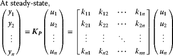
Morari applied this idea to a gain matrix relating outputs to inputs at different frequencies. It will be seen in Chapter 8 that a multivariable transfer function, for example

converts a vector of steady input oscillations at frequency ω radians per unit time to a vector of steady output oscillations at the same frequency, but with the amplitudes altered according to the gain matrix:
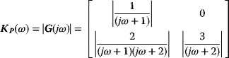
One notes that KP need not be square, and that ![]() is the steady-state gain matrix. If such a matrix cannot be inverted (or is rank-deficient), one cannot find the steady-state inputs required to achieve a particular steady-state output. This situation will vary with frequency, depending on the individual frequency responses, so the Morari resiliency index is defined for the whole frequency range as
is the steady-state gain matrix. If such a matrix cannot be inverted (or is rank-deficient), one cannot find the steady-state inputs required to achieve a particular steady-state output. This situation will vary with frequency, depending on the individual frequency responses, so the Morari resiliency index is defined for the whole frequency range as
As the MRI reduces towards zero for a particular frequency, it is understood that the system will become harder to control at that frequency. In the processing industries, one is generally interested in the steady-state gain KP(0), rather than any other frequency.
The MRI value is sensitive to the units of the individual gain entries in KP. To allow comparison of this ‘controllability’ index as variables are changed, it is necessary to normalise KP11, KP12, KP21 and so on. A value such as 0.2 °C (%open)−1 might, for example, be normalised to
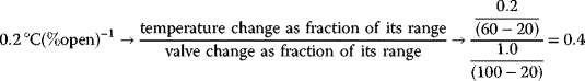
if the normal range of operation is between 20 and 60 °C, and the valve is restricted between 20%open and 100%open.
5.2.4 Relative Gain Array (Bristol Array)
In Sections 5.2.2 and 5.2.3, quantitative methods were considered to assess the controllability of part of a plant, based on the dynamic equations for the open-loop model relating inputs (proposed MVs) to outputs (proposed CVs), for example, Figure 5.5 (which is based on Figure 5.2). The methods could be applied to an entire plant, but it is likely that only difficult interactive subsections would be analysed in this way. The methods there gave no indication of how the control was to be performed.
Figure 5.5 Section of a plant from Figure 5.2 to be assessed for pairing of MVs and CVs in SISO control loops.
Particularly before the widespread use of digital computers (but even nowadays as one aims for as simple a scheme as possible), it was necessary to break down interactive plant subsections into a number of SISO control loops. The relative gain array (RGA), sometimes called the Bristol array, was developed by Bristol (1966) to identify the pairings of MVs with CVs which would minimise undesirable interactions in a system. Even simple control tasks, such as in Figure 5.6, can be susceptible to loop interaction. In this example, if the supply line has appreciable resistance, FC1 can ‘ride’ FC2 in ever-increasing oscillations as each loop attempts to compensate for the pressure variation caused by the other.
Figure 5.6 Flow control loops ‘riding’ each other due to their effects on a common supply pressure.
Bristol recognised that if one focused on a particular control loop, an indication of its interaction with other controllers could be obtained by comparing its direct open-loop gain with the gain achieved whilst all other controllers compensated. The ijth element of the RGA is thus the ratio

The numerator term is clearly the ijth element of the steady-state gain matrix KP (i.e. KP(0) above). However, the denominator term must be derived from (a square, non-singular) KP as follows:
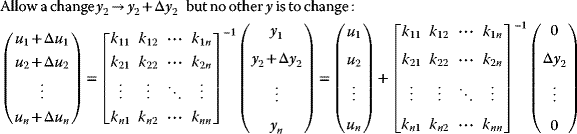
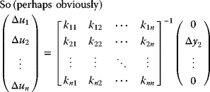
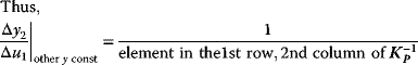

Finally, it is clear that
An element ij occurring in the RGA with a value of unity indicates that that particular pair (ith CV controlled using jth MV) would have no interaction at all with other loops. Smaller (e.g. 0.5) and larger (e.g. 2) values indicate progressively more interaction. A negative sign would imply that the sign of the controller gain has to be swopped if that loop is switched on at the same time as the other loops!
The idea of the RGA is that the control engineer would populate his or her plant with SISO loops, starting with the CV/MV pairings closest to unity. The worse pairings might still be used, but it would be sensible to make such loops progressively slower to avoid unstable interactions. Alternatively, nowadays, the engineer might deal with the more interactive combinations within a MIMO control strategy, rather than several SISO control loops.
As a caution, Luyben (1990) notes that the main requirement in the chemical processing industry is load rejection. Controllers usually regulate at fixed setpoints, and aim to minimise the effects of disturbances. Configuring a control system to minimise loop interaction does not necessarily give the best load rejection.
5.3 Control Schemes Involving More Complex Interconnections of Basic Elements
It is rare that the systematic approaches discussed in Section 5.2 are able to completely define an overall plant control scheme. Section 5.2 focussed only on the installation of SISO or MIMO controllers to meet the overall process objectives. No mention was made of the basic elements in Chapter 4 such as selectors, overrides, ratios, adders, feedforward controllers and valve position controllers which are common parts of control schemes. This Section 5.3 will illustrate how the basic elements are brought together in a few common industrial control schemes. The associated exercises, in the accompanying volume of solved problems, focus on the step-by-step interpretation of a set of instructions defining a plant control scheme. The process engineer needs a clear understanding of the process phenomena in order to properly execute these instructions. Of course, the skill one ultimately aims for is the ability to devise the overall scheme oneself, which should arise from sufficient experience with this type of specification.
5.3.1 Boiler Drum-Level Control
One of the earlier historical control schemes concerned the maintenance of a setpoint level in boiler steam drums. Figure 5.7 shows the well-known ‘three-element’ control scheme. The three elements are clearly feedback, feedforward and a supervised flow control loop.
Figure 5.7 Three-element control of boiler steam drum level.
As mentioned in Section 4.2.7, all feedforward controllers require a ‘model’, and in this case it is seen to be a very simple one, with 1 tonne of steam drawn translating exactly to 1 tonne of BFW to be supplied. Since the system integrates, and the flow measurements cannot be perfect, a feedback ‘trim’ is essential, if for nothing else, just to get the level to its initial setpoint!
The delegation of the task of maintaining a desired BFW flow rate, to a slave flow control loop, isolates the rest of the algorithm from such factors affecting the BFW flow as BFW and drum pressure fluctuations, and indeed nonlinearity of the valve itself. The direct summation of feedforward and feedback BFW demands may appear to require twice as much BFW as necessary, until one recalls that the entire algorithm is working on the basis of deviations from the initial ‘switch on’ condition.
In Section 4.2.1, it was noted that a controller acts as a ‘translator’, converting a requirement in one language (e.g. level %) into an action in another language (e.g. BFW flow t h−1). In viewing a diagram like Figure 5.7, it important to identify the implied ‘languages’ of the various signals. In particular, note that the summation involves three signals which must represent ‘t BFW h−1’.
5.3.1.1 Note on Boiler Drum-Level Inverse Response
Some processes exhibit inverse response in their open-loop behaviour. It is convenient to consider this phenomenon here, because the effect of boiler feedwater (BFW) flow on the boiler drum level is a classic example. Assume that a boiler is operating steadily, with the BFW exactly making up for the steam delivered to consumers, and the level is thus steady. The observed effects of stepping the BFW inflow up or down in this circumstance are depicted in Figure 5.8.
Figure 5.8 Shrink and swell of boiler drum level due to boiler feedwater flow variation.
Boiler feedwater will usually be de-aerated and preheated, but can in general be expected to be below the enthalpy of the equilibrium liquid in the boiler drum. Thus, an increase in the BFW flow (a), all other variables remaining constant, will cause a drop in the average enthalpy of the liquid in the drum, so that some of the immersed bubbles collapse, releasing latent heat and establishing a new equilibrium. The bubble collapse temporarily reduces the volume in the drum, and thus the level. For the case (b), where the BFW flow is decreased, additional bubbles form, as the liquid contents no longer have to compensate as much for the lower enthalpy of the BFW inflow. Clearly, these level changes would not register on a differential-pressure measurement (Section 2.4.2.1), since the level and mean density of the bubbly contents will vary as inverses.
Inverse responses of this nature, where the variable of interest temporarily ‘goes the wrong way’ after a control action adjustment, require special care in process control. In the above case (a), a controller trying to increase the level, seeing the initial drop, might try to add even more BFW, making the situation worse, and eventually over-shooting the target level. So simple controllers such as the PID (Section 4.2.4) need to be ‘de-tuned’, that is work with a lower gain KC, in order to give the level more time to respond. A predictive controller like the dynamic matrix controller (Section 7.8.2) fully anticipates the initial inverse response, allowing much tighter tuning.
5.3.2 Furnace Full Metering Control with Oxygen Trim Control
In Section 4.2.7 the maintenance of oxygen in the flue gas from a furnace was used to illustrate a purely feedforward strategy. Mention was made there of the necessity to maintain flue gas %O2 above zero to ensure combustion, but not so high as to incur significant heat loss. About 3% on a molar basis (compared to a maximum of 21% in air) seems typical industrially. If there is no actual measurement of oxygen, then a larger margin may be necessary to ensure safety.
Figure 5.9 shows the full metering control with oxygen trim control presented by Smith and Corripio (1985). This is an air/fuel ratio control with an additive feedback trim from a flue gas oxygen controller. The implication at the summer is that the feedback signal from the AC will request a zero adjustment if the ratio controller, which is working with absolute flow rates, is already achieving the setpoint %O2. This feedforward–feedback arrangement will minimise %O2 deviations from setpoint. The air flow rate controller is a slave in the cascade, whilst the fuel flow setpoint will arrive from the operator, or another controller such as the process stream TC or a boiler PC. The scheme shown includes a high and a low ‘clip’ on the air flow rate setpoint. The low clip is a good safety measure, but the high clip could lead to incomplete combustion at high fuel demands. A slight variation of this scheme is sometimes encountered where instead of supplying an additive trim to the air flow rate setpoint, the oxygen controller manipulates the setpoint air/fuel ratio RAF SP directly.
Figure 5.9 Furnace full metering control with oxygen trim control.
The scheme in Figure 5.9 has another drawback to do with the system dynamics. One notes that the fuel flow rate will always change in advance of the air adjustments, simply because there will be dynamic lag of the actual air flow as the ratio controller moves the air flow setpoint in response to the measured fuel flow variations. This situation is described as fuel leads air in and fuel leads air out. The latter situation is safe, because air will temporarily be in excess. However, the fuel leads air in is dangerous, because the implication is that there will temporarily be a deficit of oxygen.
5.3.3 Furnace Cross-Limiting Control
The dynamic lag of the air flow controller in Section 5.3.2, Figure 5.9, was seen to cause a temporary drop in the air/fuel ratio when the fuel flow increased. The cross-limiting scheme in Figure 5.10 overcomes this problem by using both measured flows to ensure a minimum air/fuel ratio at all times.

Figure 5.10 Furnace cross-limiting control to avoid decreases of air/fuel ratio below setpoint.
The cross-limiting control scheme is best explained using an example. Consider the situation where the system is initially steady maintaining the correct air/fuel ratio. Now TC1 demands an increase in fuel in order to maintain its setpoint temperature. This demand will be ignored at the LS, because the desired fuel will be higher than the allowed fuel (which initially will be the actual fuel). However, the HS will pass this higher demand rather than the actual fuel, so after multiplication by the air/fuel ratio, the air flow will start to rise to match the desired fuel. As the actual air flow rises, following its controller setpoint, the cut-off limit (allowed fuel) arriving at the LS rises in proportion, gradually allowing the fuel setpoint to increase, and ultimately the actual fuel will rise to the desired fuel. One notes that air leads fuel in, which is a safe action. Conversely, if one follows the sequence of events when desired fuel decreases, it will be found that air follows fuel out, which is again a safe action. So in any transient, there will temporarily be a safe excess of air, which will return to the correct ratio when the process settles down again.
Furnace control schemes as in Figures 5.9 and 5.10 may also have an additional safety feature to prevent flame-out. It is understandable that the fuel valve could swing to the shut position temporarily, depending on the controller gain, as it seeks to hold the flow setpoint. This would cause an irreversible situation where the flame is lost. As the valve moves open again, uncombusted fuel will accumulate in the furnace box and ducting, and may explode all at once should a source of ignition be found, for example at a neighbouring furnace sharing the same ducting. Thus, it is necessary to ensure a minimum fuel flow. This can be done using an override controller which senses the fuel pressure just before the burner nozzle. Figure 5.11 shows an arrangement where an override pressure controller maintains a minimum pressure, and implicitly a flow.
Figure 5.11 Fuel pressure override to prevent furnace ‘flame-out’.
References
- Bristol, E.H. (1966) On a new measure of interaction for multivariable process control. IEEE Transactions on Automatic Control, 11, 133–134.
- Buckley, P.S. (1964) Techniques of Process Control, John Wiley & Sons, Inc., New York.
- Johnston, R.D. and Barton, G.W. (1984) Control objective reduction in single-input single-output control schemes. International Journal of Control, 40, 265–270.
- Johnston, R.D. and Barton, G.W. (1985a) Structural equivalence and model reduction. International Journal of Control, 41, 1477–1491.
- Johnston, R.D. and Barton, G.W. (1985b) Single input-single output control system synthesis. Computers and Chemical Engineering, 9 (6), 547–555.
- Lin, R.M. and Lim, M.K. (1994) Analytical model updating and model reduction. International Journal for Numerical Methods in Engineering, 37, 1881–1896.
- Lin, X., Tade, M.O. and Newell, R.B. (1991) Output structural controllability condition for the synthesis of control systems for chemical processes. International Journal of Systems Science, 22 (1), 107–132.
- Luyben, W.L. (1990) Process Modeling, Simulation and Control for Chemical Engineers, 2nd edn, McGraw-Hill, New York.
- Morari, M. (1983) Design of resilient processing plants III: a general framework for the assessment of dynamic resilience. Chemical Engineering Science, 38, 1881–1891.
- Smith, C.A. and Corripio, A.B. (1985) Principles and Practice of Automatic Process Control, John Wiley & Sons, Inc., New York.
- Stephanopoulos, G. (1983) Chemical Process Control: An Introduction to Theory and Practice, Prentice Hall.