
3
Modelling
The most important skill that the process engineer brings to bear on the field of process control and optimisation is his/her ability to describe the dynamics and relationships of process variables. The model (Figure 3.1) may serve several purposes:
- insight and understanding;
- basis for controller/optimiser design;
- offline testing of controller/optimiser;
- basis of filter for online estimation of process variables.
Figure 3.1 General open-loop process model.
In the distant past, models sometimes ran on analogue computers – using capacitors and resistors to convert signals. However, what is being thought of here is an algorithm which will run on a digital computer. Variations to bear in mind include
- theoretical versus regressed (black box);
- continuous versus discrete equations;
- logical versus analogue;
- online versus offline;
- linear versus nonlinear;
- lumped versus distributed;
- continuous versus discrete versus mixed inputs and outputs;
- single versus multiple behaviour regimes (modes);
- numerical versus analytical solution;
- multi-input, multi-output (MIMO) versus single-input, single-output (SISO);
- differential versus algebraic;
- open loop versus closed loop;
- state-space versus input–output;
- deterministic versus stochastic;
- approximate versus accurate;
- stable versus unstable;
- transfer function form versus equation form.
In this chapter, the focus will be on the modelling of the process itself. At the outset, an important distinction should be noted between input–output model forms and recursive (or autoregressive) model forms (Figure 3.2). The former typically arise from observation of the process as a ‘black box’, whereas the latter are usually based on physical principles and involve the states of the system. Additionally, there is the idea of the process input u(t) being exogenous, meaning that it is being imposed from outside of the process. Without an exogenous input, a process cannot be controlled, so this form could only be used to describe variation from an initial state, for example decay or equilibrium processes varying towards final asymptotic states.
Figure 3.2 Basic model forms.
Most of the effort will be directed at developing the model of the process itself, that is the open-loop model without the additional effects of feedback control, optimisation or identification. When it is desired to use the model equations as the basis of a control/optimisation/identification design, one normally makes simplifying assumptions (e.g. linearisation). However, the resultant algorithms need to be tested on as accurate a model as possible. Such an accurate model may only be representable in a series of program code steps including decision points, saturation tests, clipping of negative flows and so on. The discussion that follows will attempt to be as general as possible within the above variations.
3.1 General Modelling Strategy
Control engineers are particularly interested in the dynamics of processes, that is outputs (PVs) that change over a period of time once a change occurs in a process input (MV or DV). In some situations, processes can have continuous variations (limit cycles, chaotic behaviour or instability) even if all input variations have ceased! It is the slowly responding processes (e.g. temperature of a large catalytic bed) that are particularly problematic, because it is difficult to predict exactly where they will end up. Fast processes effectively obey algebraic equations, so problems such as overshoot are insignificant. For example, one fills car tyres at the garage using a very quick feedback from the pressure gauge.
Variables that respond over a period of time store important information that is required to predict the ongoing changes in a system. If a flow is introduced to fill a tank, one needs to know the initial level in order to predict the future level variation. This type of variable is called a state of the system:
This idea is instinctive to engineers – the states are apparently those variables which have to be integrated to solve for the response. However, the set of states may not be unique, and may include discrete variables, such as the status of a bursting disc resulting from a past state value. The tank level and flow system in Figure 3.3 has some of these features.
Figure 3.3 Tank with two restricted outflows and a bursting disc.
The dynamic modelling of a system like this is best tackled in several steps:
- Determine which variables are constant and which could vary in time.
In this example, the only time-varying quantities are f1, f2, f3, h and b. There is no indication that the flow coefficients k1, k2, k3 (see below), H and Hb are likely to change.
- Determine which of the time variables are independent inputs (MV or DV, possibly discrete), and which of the rest, if any, should be chosen as states.
Here f0 is an independent input. h is an obvious state, because its starting value is required to predict its future values. On reflection, that would not be enough, as the starting value of b would be required as well. In fact, the starting values of both h and b are required to predict all future values of both h and b, provided the input f0(t) is known for t > 0. So a sufficient set of states is {h, b}. In this problem, an alternative selection of states may be made, namely {f1, b}. This is made possible by the monotonic algebraic relationship between f1 and h. The particular choice of states in a given problem will depend on the focus. If the focus is on the implications of the varying exit flow f1, this might well be chosen as a state instead of h.
- For each continuous state variable, use a balance of the form ‘Accumulation = In − Out’ to obtain its time derivative.
The dynamic balance will normally involve mass or energy, or possibly momentum. Often the equations will involve other states, meaning that the system is ‘coupled’ or ‘interactive’. Typical items involved in balances are listed in Table 3.1.
In the present example, the volume balance gives
since the liquid surface area in the vessel A is constant.
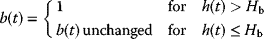
- For each discrete state variable, determine the logic governing its value.
(3.2)
- The remaining time variables (ancillary variables), which are neither states, nor MVs nor DVs (but which could be discrete), must be related to each other and the states, MVs and DVs using algebraic and logical expressions.
Following the discussion in Section 2.4.1.1, for a fixed liquid density one can take
(3.4)
- A stepwise solution can then be set up for the period 0 to tf using a simple Euler integration.
Table 3.1 Typical quantities involved in dynamic balances.
| Extensive property | Accumulation rate | Inflows | Outflows | Units of balance |
| Mass | dW/dt | Streams in | Streams out | kg s−1 |
| Reaction generation | Reaction consumption | |||
| Desorption, permeation, diffusion, evaporation and so on | Absorption, permeation, diffusion, evaporation and so on | |||
| Moles A (one species in a flow) | dmA/dt | Streams in | Streams out | kg mol A s−1 |
| Reaction generation | Reaction consumption | |||
| Desorption, permeation, diffusion, evaporation, dissolution and so on | Absorption, permeation, diffusion, evaporation, crystallisation, filtration, precipitation and so on | |||
| Volume (liquids) | dV/dt | Streams in | Streams out | m3 s−1 |
| Permeation, condensation and so on | Permeation, evaporation and so on | |||
| Energy | d{ρVcPT}/dt | Streams in (enthalpy) | Streams out (enthalpy) | kW |
| Exothermic reaction heat | Endothermic reaction heat | |||
| Transfer in (convection, conduction, radiation) | Transfer out (convection, conduction, radiation) | |||
| Mechanical work | Evaporation, melting | |||
| Condensation, freezing | Heat of solution (endo) | |||
| Heat of solution (exo) | ||||
| Momentum | W d2y/dt2 | Applied forces | Friction | kg m s−1 |
| Shear | Potential |
Several aspects of the above procedure (steps 1–6) should be noted. Real problems will always involve logical tests, whether they be for empty or overflowing tanks, limits of valve ranges or signal saturation. Since the solution is typically performed as a series of computer statements, there is no point in attempting to eliminate variables, for example by substituting Equations 3.3–3.5 into Equation 3.1. In fact, one would lose useful information by doing this. Another point is that the algorithmic approach in Figure 3.4 easily adapts to real-time implementations by synchronising the timing loop. More sophisticated integration schemes can be substituted once the basic algorithm works, but modern computer power does not warrant a lot of effort on this aspect.
Figure 3.4 Stepwise algorithm for open-loop system in Figure 3.3 using Euler integration (note: ‘=’ implies assignment).
In the processing industries, there are many problems that are well described by a set of DAEs (differential and algebraic equations). Typically, the lumped differential part describes accumulations in vessels, and the algebraic part describes stream interconnections. The algebraic equations may be implicit (i.e. the dependent variable appears on both sides of the equation), and in any case, the differential equations become very unwieldy if substitutions are attempted to get a set of differential equations alone. Thus, many workers have developed software for solution (integration or optimisation) of a system described by DAEs. The above integration solution for the simple tank problem might appear not to warrant anything more sophisticated. It seems in this example that most complications could be dealt with just by decreasing the step size Δt. But in general the algebraic equations could be implicit, and there could be a large set of coupled DEs, possibly with problems of stiffness (fast and slow responses together). Moreover, in an optimisation mode, one might, for example, seek the best f0(t) variation to bring h to its setpoint (SP), so the equations have to be solved more or less backwards.
However, the preceding discussion of DAE solutions applies to systems which have no logical equations. It has been noted above that real systems will in general require description by what one might call DALEs (differential, algebraic and logical equations). Certainly that was the case in the tank example above. The effect of the logical equations is to create discontinuities in the functions describing the behaviour. A few workers such as Mao and Petzold (2002) have developed integration solutions for DALE systems. However, the optimisation problem is difficult because of the branching caused by the logical expressions. Typically, a MINLP (mixed integer nonlinear programming) solution is required in a commercial package such as GAMS®.
Define vectors x to contain all of the continuous states, w the discrete states, y the ancillary variables and u the input MVs and DVs. It is noted that y and u may contain both continuous and discrete variables. The integration problem amounts to solving
for a given ![]() , where f and g are vectors of functions. On the other hand, a typical constrained optimisation problem might involve for
, where f and g are vectors of functions. On the other hand, a typical constrained optimisation problem might involve for
find ![]() , such that
, such that ![]() and
and ![]() is minimised.
is minimised.
Here the vector of functions h represents the constraints, whilst the scalar function ϕ is the objective function for the optimisation.
3.2 Modelling of Distributed Systems
There are many instances of distributed systems in the process industries. This is where conditions vary with both time and position, requiring the system to be described using partial differential equations (PDEs). Examples include reactors which are not mixed, packed absorption, extraction and distillation towers, fixed bed leaching and filtration, and heat exchangers. Usually one is interested in conditions at the exit of such equipment, but quite often there is interest also in values at intermediate positions. Regardless, the only way to model the behaviour is by solution of the PDE. This is usually done by discretisation in the spatial dimensions, such as x in the axial flow reactor in Figure 3.5. So instead of modelling just one value of CA, now one has to model n values just to get the one or two results required. This confirms the idea that the state CA has become distributed. The approximate solution based on discretisation effectively creates n lumped states CA1, CA2,…, CAn and these must be solved simultaneously using the resultant n ordinary differential equations (ODEs). Mathematicians have developed various schemes for these solutions (ADI, Crank–Nicholson, tridiagonal), but in Figure 3.5, a simple sequential Euler integration is again shown which ignores changes in neighbouring elements during each time step.
Figure 3.5 Lumped and distributed systems: mixed flow and axial flow reactors.
One notes that the one-dimensional discretisation procedure shown divides up the volume into n completely mixed compartments, that is the ‘tanks-in-series’ model. The greater the value of n, the more closely the plug flow is approached. Actually, n can be set to simulate a degree of axial dispersion according to n = Lu/DA approaching plug flow for large n (>50) and approaching mixed flow for small n (n = 1 being ideal mixed flow). In this expression, L is the length of the flow path, u is the superficial velocity and DA is the (axial) eddy diffusivity in the flow direction.
In the processing industries, dead time, also known as ‘transport lag’, is a common phenomenon related to distributed systems (Figure 3.6). This is typically caused by flow through long pipelines, or large volumes that are unmixed. Another source of dead time is travel on conveyor belts. To model dead time dynamically, one could follow the same procedure as for the axial flow reactor in Figure 3.5, without any reaction of course. A large number of compartments, and thus states, would be required to avoid serious blunting of the shapes of signals passing through. A typical computer algorithm for achieving a pure delay is given in Figure 3.7. A cyclical (‘wrap-around’ or ‘stack’) file is achieved by the pointer jumping back to the start, once it reaches the end. When the delayed value is found by moving backwards from the pointer, interpolation could be used to improve the ‘looked-up’ value. The file must be long enough to handle the longest expected delay, or at least the oldest value should be returned for an unusually long delay (e.g. zero flow).
Figure 3.6 Transport lag (dead time).
Figure 3.7 Use of a cyclical file and moving pointer to simulate a transport lag.
3.3 Modelling Example for a Lumped System: Chlorination Reservoirs
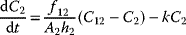
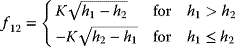
Consider the pair of drinking water conditioning reservoirs in Figure 3.8. The treated water enters the first reservoir at flow f0 and with chlorine concentration C0. An interconnecting pipe between the two reservoirs transfers water either way (‘tidal flow’), depending on which level is lower, which is determined by the rates f1 and f2 at which water is drawn from each compartment, as well as the feed rate f0. Assuming that each reservoir is well mixed, the varying levels and flows will cause a varying residence time, and thus a varying residual chlorine content at each exit, since the dissolved chlorine is gradually lost.

Figure 3.8 Interconnected chlorine conditioning reservoirs for drinking water.
The problem posed is to develop an algorithm for prediction of the behaviour of this system over a period of time, t = 0 to t = tf.
Solution:
- Variables:
h1(t), h2(t), C1(t), C2(t) continuous states f0(t), C0(t), f1(t), f2(t) continuous MVs and DVs f12(t), C12(t) ancillary continuous variables k first order rate constant for chlorine decay K constant coefficient for pipe flow A1, A2 constant water surface area in each reservoir - Volume balances:
(3.14)
 (3.15)
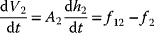
- Chlorine balances:
(3.16)
 (3.17)
- so
(3.18)
 (3.19)
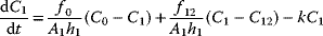 (3.20)
 (3.21)
- so
(3.22)
- Algebraic equations:
(3.23)
 (3.24)
- The algorithm is given in Figure 3.9.
Figure 3.9 Stepwise algorithm for open-loop reservoir system in Figure 3.8 using Euler integration (note: ‘=’ implies assignment).
3.4 Modelling Example for a Distributed System: Reactor Cooler
Figure 3.10 shows the combined reactor and cooler used in the BASF process for formaldehyde production from methanol. The reaction gases pass through a 2 cm thick catalytic bed lying on a perforated crucible. As the reaction product gases enter the tubes of the cooler, they are around 650–700 °C, and must be cooled rapidly to avoid the formation of by-products. Boiler feed water is fed through an equal-percentage valve at the bottom of the shell side of the cooler. As the water moves up, it becomes steam at some point, and the steam is allowed to proceed to users through an equal-percentage valve connected to the top of the shell.
Figure 3.10 Reactor crucible and tubular cooler for BASF process: formaldehyde by dehydrogenation of methanol over silver catalyst.
Since both the reaction gas side and the water/steam side are distributed, the cooler will be represented by a series of elements (1,…, N) as in Figure 3.11, which interconnect the two sides by virtue of a heat transfer surface.
Figure 3.11 Conversion of distributed system into multiple lumped systems by discretisation of spaces for reaction gas, water and steam for reactor cooler in Figure 3.10.
The art of creating a model is (a) to record as many equations as possible which interrelate the variables and (b) to recognise reasonable approximations which simplify the model as far as possible.
To simplify the solution on the water/steam side, the following assumptions will be made:
- Water enters at its boiling point, which is determined by the steam pressure.
- Sensible heat transfer to the water is negligible – all heat added creates steam.
- Steam bubbles rising in the water occupy little volume.
- The water volume is well mixed.
- The steam volume is well mixed.
- The variation of cP with temperature is ignored.
- Mass flows WG (gas moving down) and WS = WW (steam/water moving up) are taken constant with height.
Solution:
- Variables:
xW(t), xS(t), TG0(t), WG(t) continuous MVs and DVs PW, PU pressures of BFW supply and steam users assumed constant α, β, kW, kS valve characteristic constants and flow coefficients AG, AW, a constant flow areas and heat transfer area per unit height UW, US constant overall heat transfer coefficient from gas to water and gas to steam ρW, cPW, cPS, cPG, λ constant properties of fluids (including latent heat) A, B, C constant Antoine coefficients for water PS(t), TS(t), hW(t) single continuous state variable: pressure on water/steam side, temperature of steam, height of water For each element ‘i’ TGi(t) continuous state variables: temperatures of reaction gas qi(t) ancillary time-dependent variable: heat transferred from reaction gas to water/steam in element i - Water level:
(3.25)

- Energy balances:
(3.26)
 (3.27)
 (3.28)
- Steam balance (with molecular mass MS = 18):
(3.29)
 (3.30)
- Algebraic equations:
(3.31)
 (3.32)
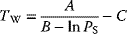 (3.33)
 (3.34)
for ‘TGN+1’ use TG0.
The algorithm is given in Figure 3.12.
Figure 3.12 Stepwise algorithm for open-loop distributed reactor cooler system in Figure 3.10 using Euler integration (note:  implies assignment).
3.5 Ordinary Differential Equations and System Order
The modelling problems considered so far have been somewhat ‘open-ended’, requiring rather ad hoc approaches. It was intended merely to obtain as close a representation of the physical phenomena as possible, bearing in mind that the algorithmic approach (sequential computer instructions) gave a lot of freedom to deal with state-dependent behaviour, discontinuities, logical/discrete issues, saturation and nonlinearity. The models developed were based on physical principles, giving access to meaningful parameters (e.g. heat transfer coefficients) which could be adjusted to get a good match to real plant behaviour. It is a good idea to develop skills in this type of algorithmic modelling, because it allows one to simulate real process behaviour more closely.
Moving on from the strictly algorithmic approach, it needs to be recognised that the useful theoretical ideas that are going to be developed later in this text for control, identification and optimisation will usually rely on more restricted types of models – typically those that can be expressed directly as a set of first-order ODEs. (In fact, a lot of useful ideas are based on the specific case of a system of linear ODEs.)
The order of a system is the number of equations using a first derivative (d/dt) that one needs to represent its dynamics. In other words, following on from Section 3.1, the order is determined by the number of states. In the lumped chlorination reservoir problem of Section 3.3 it was 4, and in the distributed reactor cooler problem of Section 3.4 it was N + 2. (So the process of discretising the spatial dimension of a system described by PDEs leads to extra states, and an increase in order by the same amount.) In the processing industries, virtually all of the individual differential equations found in mass and energy balances for lumped systems will arise as first derivatives. There are a very few situations where this type of theoretical modelling of physical phenomena leads initially to a second-order differential equation. Usually this is where there is inertia and momentum involved, for example compressor shaft rotation, pipeline flow or mercury in a manometer. To illustrate this point, consider the well-known mechanical mass, spring and dashpot example in Figure 3.13
Figure 3.13 Force applied to trolley with spring and dashpot resisting.
A force balance leads to the equation
that is
which is the standard form of a second-order system, where
This system has two states, namely ![]() , velocity, and x2 = y, position. Initial values are required for both of these in order to solve for the continued variation of the system with F(t). Equation 3.36 can then be written as the system of first-order ODEs
, velocity, and x2 = y, position. Initial values are required for both of these in order to solve for the continued variation of the system with F(t). Equation 3.36 can then be written as the system of first-order ODEs
where
and since this happens to be linear it can be expressed as
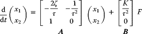
which is clearly a second-order system. Obviously, if independent differential equations arise in the modelling, these can be solved separately. However, the higher order systems one is contemplating here are those that have interdependent differential equations, that is they share the state variables x1, x2,…
More generally, the ‘state-space’ representation of a continuous system (Figure 3.14) is
and if it happens to be linear one can use the common form
Referring to Section 3.1, one notes that Equation 3.44 is a special case of Equations 3.6–3.9, with no ancillary algebraic equations and variables shown. A form like Equation 3.44 could of course still be obtained from Equations 3.6–3.9 where ancillary algebraic equations exist, provided all of the ancillary variables could be eliminated from the expression by substitution.
Figure 3.14 General state-space system.
3.6 Linearity
In process control one spends a lot of time thinking about linearity, because most of the robust and powerful methods assume linear process behaviour. One needs to be able to find linear versions of process models and to deal with the problems of mismatch to the actual process.
As in Section 3.1, let vector x contain the continuous states, y the ancillary variables and u the input MVs and DVs. With the restriction that discrete states cannot be considered, nor discrete variables in y and u, the system of Equations 3.6–3.9 becomes
where f and g are vectors of continuous functions. Considerations of linearity will focus on the input–output relationship u(t) → x(t) (Table 3.2).
Table 3.2 Principles of linearity.
| Principle | Implication | Responses |
| Superposition | If u1(t) → x1(t) and u2(t) → x2(t), then [u1(t) + u2(t)] → [x1(t) + x2(t)] |
|
| Homogeneity | If u1(t) → x1(t), then a × u1(t) → a × x1(t) |
|
| Stationarity | If u1(t) = A sin(ωt), then eventually x1(t) will be sinusoidal with the same frequency ω |
|

Figure 3.15 Tank with restriction orifice at exit.
Two examples will serve to illustrate the test for linearity by superposition.
Note: According to the principle of superposition, it would appear that an equation like
is nonlinear. However, it is noted that it is easily linearised by substituting either a new input variable w = u − 2 or a new state variable ![]() .
.
3.7 Linearisation of the Equations Describing a System
Again, the discussion here will focus on continuous systems which do not involve discrete states or inputs, that is as in Equations 3.46–3.47:
Define a Jacobian matrix symbolically ![]() as
as

and similarly for ![]() , but it is noted, however, that the latter Jacobian matrices will not in general be N × N. Choosing a point (x0, y0, u0), where f = f0 and g = g0, about which to perform the linearisation, a Taylor series expansion to the second term yields
, but it is noted, however, that the latter Jacobian matrices will not in general be N × N. Choosing a point (x0, y0, u0), where f = f0 and g = g0, about which to perform the linearisation, a Taylor series expansion to the second term yields
Using deviation (‘perturbation’) variables ![]() ,
, ![]() and
and ![]() , and choosing the point (x0, y0, u0) such that it satisfies g(x0, y0, u0) = 0 and causes the system to lie at steady state, that is f(x0, y0, u0) = 0,
, and choosing the point (x0, y0, u0) such that it satisfies g(x0, y0, u0) = 0 and causes the system to lie at steady state, that is f(x0, y0, u0) = 0,
To resolve the ancillary variables, ![]() has to be square and nonsingular, so
has to be square and nonsingular, so
which on substitution in Equations 3.68–3.69 yields the linear equation
where
In many situations, the nonlinear or implicit form of g does not permit easy substitution (prior to linearisation). So it is worthwhile remembering that separate linearisation of Equations 3.68–3.69 as above leads to the same result.
Figure 3.17 Tank with restriction orifice at exit.
Example 3.3 follows the general procedure without a direct substitution of the ancillary variable F1 in the original differential equation, which, as mentioned, is often problematic. Furthermore, in the process of assuming a steady-state point (h, F1, F0)0 which satisfies g = 0, it is important to identify the implications:
So ![]() represents deviations from the steady-state inflow F00. Moreover, if it required to establish the actual absolute level in the tank for a particular h′ value, it must be added back to its offset, namely h = h′ + h0.
represents deviations from the steady-state inflow F00. Moreover, if it required to establish the actual absolute level in the tank for a particular h′ value, it must be added back to its offset, namely h = h′ + h0.
In this example, the linearisation entails an approximation for F1 as represented in Figure 3.18.
Figure 3.18 Linearisation of orifice flow characteristic for tank flow example (Example 3.3).
3.8 Simple Linearisation ‘Δ’ Concept
At the risk of repeating what has already been recommended in Section 3.7, it is worth suggesting an equivalent ‘delta’ procedure for linearisation of systems of DAEs. Taking the restricted case of the continuous system
(which has no discrete variables or ‘logical’ mode changes), one recognises that
where ‘Δ’ represents the linear partial derivative chain with respect to all of the time variables present in any term. Bearing in mind the assumption of linearisation about the steady-state operating point, one simply passes the Δ operator through all of the available differential and algebraic equations. The equivalent treatment of Example 3.3 is then as in Example 3.4. Again, it must be remembered that implicitly the resultant new deviation (or perturbation) variables ![]() are deviations from a particular set of values
are deviations from a particular set of values ![]() which cause
which cause ![]() and
and ![]() .
.
3.9 Solutions for a System Response Using Simpler Equations
In the lumped and distributed system examples of Sections 3.3 and 3.4, stepwise algorithmic approaches were used to obtain the output response to time variations of the input MVs and DVs. Special logical tests were required in the integration cycle t → t + Δt to handle such occurrences as state-dependent changes in behaviour. In dynamic systems, these solutions are clearly integrations of the defining equations. In many cases, it is satisfactory to consider operation in a restricted range where variables can be treated as unbounded (no saturation) and no logical branches need to be handled. Most control systems are based on models where such assumptions have been made, usually with an additional assumption of linearity. It is worthwhile to consider several forms of mathematical solution of such systems, because (a) the resultant formulae are often useful, and (b) some ideas arising in these solutions form part of the conceptual basis and language of control theory. So, at the outset, consider a linear system described by the general form of Equations 3.70–3.72:
Here the ‘prime’ has been dropped from the time-variable vectors x(t), u(t) and y(t) for convenience, as is common practice, but one must obviously remain conscious that the values are deviations from the steady-state condition. In certain systems, the matrices A, B, C and D can be time dependent, but that case will not be considered here. It is noted that A is an N × N matrix, where N is the order of the system, that is the number of states needed to describe it. The matrix B is N × M, where M is the number of inputs to be considered (MVs and DVs). Any number P of ancillary ‘output’ variables y may be involved, with C and D being P × N and P × M, respectively. The latter concept is often useful when the only measurable observation or feedback is based indirectly on the states, for example ‘weighted average bed temperature (WABT). Often it is not possible to observe all of the states x, in which case one is considering an input–output system ![]() , where y is a (linear) combination of some selection of the states.
, where y is a (linear) combination of some selection of the states.
3.9.1 Mathematical Solutions for a System Response in the t-Domain
One system readily lending itself to time-domain solution is the SISO case of Equation 3.100:
where a and b are merely scalar constants. In the case of the tank flow example (Example 3.3), it was seen that
Integration of Equation 3.102 is possible for certain forms of u(t) by separation of variables. Noting that
it follows that
Integrating from 0 to t
so
Two specific cases are considered in Table 3.3.
Table 3.3 Time-domain response solutions for a first-order linear system.
| Input | Solution | Output response plot |
| u(t) = 0 for t > 0 | where a is negative for stable systems (else unlimited growth) |
|
| u(t) = α (const) for t > 0 |  (a is negative for stable systems) |
|
Moving on to a second-order system with constant coefficients A and B, the time-domain solution becomes more difficult, and is developed as the sum of a complementary solution (u(t) = 0) and particular solution (u(t) ≠ 0). For such larger linear models, it will be found easier to obtain output responses using Laplace s-domain methods in the next section.
3.9.2 Mathematical Solutions for a System Response in the s-Domain
Laplace transform methods using the parameter ‘s' are seldom used in the processing industries, yet they are very important on a conceptual level. A lot of the useful theory refers to aspects of these methods, whether the context involves ‘pole locations', ‘frequency response', ‘stability margins', ‘transfer functions' or ‘integrators'. It will be found that a good background in these methods enables one to build up a mental picture of key aspects of process dynamics and control.
3.9.2.1 Review of Some Laplace Transform Results
The Laplace transform of a function of time x(t) is defined as
Only behaviour at times t ≥ 0 is considered, so it is implicit in the approach that all time functions are zero up until t = 0.
Apart from the fact that s-domain versions of various functions may be found in tables, one notes that the operator L{·} is linear, so that if ![]() , then
, then ![]() . Furthermore, Laf(t)} = aF(s).
. Furthermore, Laf(t)} = aF(s).
Now consider the transform of the time derivative:
Integrating by parts
A similar treatment for the second derivative yields
In general, provided ![]() for
for ![]() , then
, then
For integration, note that
These results will shortly prove useful for the conversion of ODEs with constant coefficients into transfer functions. However, transport (dead-time) lag (Figure 3.19) cannot be described using ODEs, and warrants a special treatment.
Substituting ![]() ,
,
So the transfer function of a dead-time lag τT is
Several useful Laplace transform results are summed up in Table 3.5.
Figure 3.19 Transport lag (dead-time lag).
Consider an arbitrarily high-order SISO linear system with constant coefficients similar to the trolley with spring and dashpot in Section 3.5.
Consider the particular circumstance of
This requires that the system starts at t = 0 with both input u and output x at zero, and at a ‘complete' steady state where the indicated time derivatives are all zero. Then Equation 3.120 gives
Thus, in the s-domain, a transfer function G(s) can be used as a multiplier to represent Equation 3.129.
For a system to be physically realisable, it is necessary that n ≥ m. Indeed, in the trolley, spring and dashpot example of Section 3.5, n = 2 and m = 0. Few physical systems would be modelled with the derivative terms on the right-hand side of Equation 3.129. Mathematically, one might propose a system like
but one would be asking for an impossible response, for example if u were a step function.
The standard input function transforms in Table 3.4 suggest that, in general, the input U(s) would be expressed as a ratio of two polynomials in s. Since the transfer function G(s) in Equation 3.133 is similarly a ratio of two polynomials in s, one expects that usually the output X(s) will arise as a ratio of two polynomials in s. These will be more complex than the simple transforms in Table 3.4, so they must be broken down into more elemental pieces using a partial fraction expansion.
Say
Letting
where qi, i = 1,…, k, are the roots obtained by setting the denominator to zero. If these roots are all distinct, one can write
Otherwise, if a root is repeated – say q1 occurs three times – write
In the case of distinct roots, one multiplies by each denominator factor in turn, and simultaneously sets s to the root value, for example
For the repeated roots, first multiply by the highest power denominator
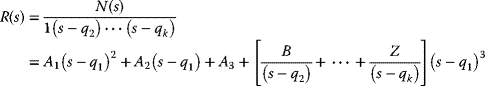
Now obtain
In general, s is a complex number, and complex roots qi certainly can arise in the above procedure. These are associated with oscillation in the response. Such roots will occur in complex conjugate pairs, and the associated coefficients must then also be expected to occur in complex conjugate pairs so that the complex variable ![]() does not remain in an expression like Equation 3.139 if a real value of s is substituted.
does not remain in an expression like Equation 3.139 if a real value of s is substituted.
Say
Then it is required that ![]() so that
so that
which is real for real s.
Going a little further, one notes that Tables 3.4 and 3.5 allow the following inversion (L−1{·}) of these first two terms of the expansion to the time domain:
Note that it is implicit in all of these developments that s, a and b have units of inverse time. In the angular sense this is understood as radians per unit time.
The above discussion is based on the premise that the function to be inverted will occur as a ratio of two polynomials in s. One notable exception to this occurs with the transport lag G(s) = e−τs in Table 3.5. If this is simply a multiplier of the expression, it can be used subsequently to time shift the result. If it is embedded, special procedures such as the Padé approximation will be required (Section 8.2.1.1).
Table 3.4 Selected Laplace transforms.
| x(t) | Plot | X(s) |
| δ(t) | 
|
1 |
| 1 | 
|
|
| t | 
|
|
| e−at | 
|
|
| sin(ωt) | 
|
|
| cos(ωt) | 
|
Table 3.5 Selected Laplace transform results.
| First derivative | |
| Second derivative | |
| Integral | |
| Transport lag | |
| s associated with a | |
| Complex conjugate partial fractions | 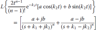 |
| Final value theorem |
3.9.2.2 Use of Laplace Transforms to Find the System Response
Now consider the use of Laplace transforms in solution of the modelling problem represented by the linear state equation (Equation 3.100).
If the elements of the matrices A and B are constant, transformation using the result (Equation 3.118) yields
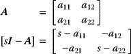
The matrix of time functions resulting from the first inversion ![]() is known as the state transition matrix (or ‘matrix exponential'– Section 3.9.3.2) and the result of its multiplication with the numerical vector of initial values x(0) will be the complementary solution. One can get an idea of the structure of the state transition matrix by examining a 2 × 2 system:
is known as the state transition matrix (or ‘matrix exponential'– Section 3.9.3.2) and the result of its multiplication with the numerical vector of initial values x(0) will be the complementary solution. One can get an idea of the structure of the state transition matrix by examining a 2 × 2 system:
Recall that
where
where

and the ![]() are minors, that is the determinant of what is left after eliminating row i and column j.
are minors, that is the determinant of what is left after eliminating row i and column j.

where the mij are the original elements of M. Applying this to [sI − A] obtain

So the complementary solution xC(t) (for u(t) = 0), given ![]() , requires evaluation of
, requires evaluation of

Each term arises as a ratio of two polynomials in s. It has been noted in reference to Table 3.4 that the terms in the forcing vector U(s) in Equation 3.151 will likewise be ratios of polynomials in s. Thus, the particular solution xP(t) (for u(t) ≠ 0 but x(0) = 0) will be similar to Equation 3.159 with larger polynomials. The final solution x(t) = xC(t) + xP(t) requires inversion of these expressions using the partial fraction expansion methods presented in Section 3.9.2.1.
The idea of a transfer function for linear systems with constant coefficients was built up in Section 3.9.2.1 based on a SISO system. Now one sees that it easily extends to MIMO systems for the case x(0) = 0 (Figure 3.20). Then the state Equation 3.151 becomes the input–output form
that is
Following Equation 3.154, note that a single scalar polynomial
will apply as a denominator throughout this transfer function, and that the adjoint matrix of ![]() , multiplied by B, will yield the set of numerator polynomials N(s), expressed here as a constant coefficient matrix for each power of s, that is
, multiplied by B, will yield the set of numerator polynomials N(s), expressed here as a constant coefficient matrix for each power of s, that is
that is
where
and the λi are clearly the eigenvalues of A.

Figure 3.20 Representation of a general SISO or MIMO input–output transfer function.
Since in the above development x contains all of the states, the requirement that x(0) = 0 implies complete steady state at t = 0.
More general linear input–output forms may not involve all of the states (Figure 3.20). These are stated directly as
From Equation 3.71 for linear systems, ![]() can effectively arise as some combination of
can effectively arise as some combination of ![]() and
and ![]()
Though input–output forms are usually not derived like this, one clearly expects from Equation 3.168 that the transfer function ![]() for this state-based system will be a similar matrix of polynomial ratios, with the denominator factors for this state-based system arising similarly from the same root values of
for this state-based system will be a similar matrix of polynomial ratios, with the denominator factors for this state-based system arising similarly from the same root values of ![]() (i.e. the characteristic equation of the state open-loop system). However, this is not generally the case for input-output systems, where arbitrary polynomial ratios can occur in G′, requiring more di and Ni terms (see Section 7.8.1)
(i.e. the characteristic equation of the state open-loop system). However, this is not generally the case for input-output systems, where arbitrary polynomial ratios can occur in G′, requiring more di and Ni terms (see Section 7.8.1)
The following examples illustrate the use of Laplace transforms to obtain the output response functions of several systems, for some standard input excitation functions. The response to an oscillating input is dealt with later in Chapter 8, for example Example 8.4.
3.9.2.3 Open-Loop Stability in the s-Domain
The idea of stability becomes very important when controllers are left in charge of a process, and this will be considered in detail later (Chapter 8). The problem is that closing a control loop around a process invites a number of problems, for example overreaction to a disturbance. For the meantime, just the open loop will be considered. Most processes are quite well behaved on their own (in open loop); for example, in all of the tank flow examples in Section 3.9.2.2, if the inflow is stepped up, the levels will rise until the exit flows balance the new inflows, where a new equilibrium is found. However, a few naturally unstable systems exist in the processing industries – notably cooled or heated reactors (exothermic or endothermic). Reaction rates are strongly dependent on temperature according to the Arrhenius relationship for rate constants:
so if the cooling is reduced on an exothermic reactor, the temperature increases, giving higher reaction rates, and thus even more heat is generated, so temperature increases rapidly and a runaway reaction occurs (provided the reagent supply is sufficient). Conversely, an endothermic reaction will die if heating is reduced.
The formal definition of stability is as follows:
The important thing is that if just one finite input function can be found that causes unbounded growth of the output, then the system must be declared unstable. An example of this would be a bridge or chimney that might only resonate in its vortex street at a particular wind speed.
The open-loop MIMO systems considered in Section 3.9.2.2 were of the forms
For these systems derived from the state equation it was noted that both transfer functions involve denominator factors based on roots of the characteristic equation of the state system, namely ![]() , that is the eigenvalues λi of A. The system itself thus contributes corresponding partial fractions to any response, in the form of factors exp{Re(λi) × t}. It is thus clear that the eigenvalues of A must all have negative real parts for open-loop stability (Figure 3.28). More generally, for input–output systems, the denominator factors in the elements of G′(s) in Figure 3.2a can all differ, giving more factors (s − ai) requiring Re(ai) < 0 for open-loop stability.
, that is the eigenvalues λi of A. The system itself thus contributes corresponding partial fractions to any response, in the form of factors exp{Re(λi) × t}. It is thus clear that the eigenvalues of A must all have negative real parts for open-loop stability (Figure 3.28). More generally, for input–output systems, the denominator factors in the elements of G′(s) in Figure 3.2a can all differ, giving more factors (s − ai) requiring Re(ai) < 0 for open-loop stability.

Figure 3.28 s-domain characteristic equation roots (stable: λ1, λ2, λ3; unstable: λ4, λ5, λ6).
3.9.3 Mathematical Solutions for System Response in the z-Domain
The continuous mathematical descriptions of a process considered in Section 3.9.1 (t-domain) and Section 3.9.2 (s-domain) are useful starting points for development of the control, identification and optimisation ideas of importance in the processing industries. In practice, of course, only an analogue computer or controller could deal with a process on this basis, and some degree of discretisation is necessary in modern monitoring and control systems. The sequence of events in these systems is much like the general algorithms presented in Section 3.1 (Figure 3.29). There are a number of timing and synchronisation issues to be considered in a real-time program like this. The main loop will execute at reasonably small intervals Δt, but it would be wasteful to execute all of the tasks on every pass. Usually sampling intervals (‘scan cycles') are set individually depending on the speed of variation of individual variables. Variables with long responses and their associated controllers will execute infrequently, whilst the continuous and logical variables in safety trip systems will be scanned in and out on a rapid cycle (or trigger ‘interrupts').
Figure 3.29 Typical timed loop of tasks on a plant computer.
There are some mathematical implications for sampled data systems like this. Chief of these is that the computer settings going back to the plant move in a series of steps. This effect would be minimal for fast sampling, and the continuous theories would apply quite well. However, there are frequently situations where data are only updated on large intervals (e.g. gas–liquid chromatograph measurements) or a control algorithm must work on a large interval (e.g. dynamic matrix control, Section 7.8.2). Moreover, since new data are only being reconsidered at discrete times, there is no point in repeating calculations between these times. Sampled data systems' theory and representations based on the z-transform allow one to properly describe behaviour from one sampling instant to the next, and to derive and analyse useful recursive formulae for real-time implementations.
3.9.3.1 Review of Some z-Transform Results
The initial requirement is to develop a formal way of describing a time series of sampled values. This is more or less just a vector of numbers to which a new value is added at each sampling instant. It is conceptually useful to represent these numbers as a series of delayed Dirac impulses of size numerically equal to the original signal values at the time instants. In Figure 3.30, some license has been taken to represent these impulse sizes by the heights of equal-base triangles. So the sampled signal then becomes the impulse-modulated function
To transform this to the s-domain, one makes use of the transport (or dead-time) lag e−Ts (Table 3.5) to delay the impulses successively. It is also noted in Table 3.4 that the δ(t) transforms to 1.
The idea of z-transforms arises from the substitution
which is just a single forward time shift in the s-domain. Then the notation x(z) is used for the transform ![]() of the impulse-modulated signal, so that
of the impulse-modulated signal, so that
A simple example would be a unit step at t = 0 (Figure 3.31).
Figure 3.30 Representation of sampled values as a series of proportional impulses.
Figure 3.31 Impulse modulation of a unit step at t = 0.
Here
Some additional useful z-transforms and their corresponding Laplace transforms are included in Table 3.7. Some care must be taken in the use of these functions. The z functions are merely s-domain functions in disguise (where z replaces eTs). In particular, the x(z) functions in Table 3.7 are the Laplace transforms of the impulse-modulated signals, and only ‘represent' the smooth functions such as t and e−at at discrete points in time. The transformation operator Z{·} implies that the argument is to be replaced by the corresponding z function from this table.
Table 3.7 Selected z-transforms and corresponding Laplace transforms.
| x(t) | x(z) | X(s) | Plot |
| δ(t) | 1 | 1 | 
|
| 1 | 
| ||
| t |

| ||
| e−at |

| ||
| sin(ωt) |
| ||
| cos(ωt) |
| ||
| Delay nT | e−nTs |

| |
| Zero-order hold of F(s) |
|
To use the z notation to solve for the way continuous signals move through a system, one needs to ‘hold' values between the impulses. The most common way of doing this is by means of the ‘zero-order hold', which keeps the signal constant at the last value, rather than trying to interpolate or extrapolate it in some other way according to higher order holds.
Consider the general signal of Equation 3.235:
that is
The zero-order hold transfer function is
Then
The term in square brackets is seen to be a unit step of +1 delayed until t = iT with an equivalent unit step at t = (i + 1)T subtracted from it after an interval of T. The resultant square pulse is also scaled by its own factor x(iT). All of these functions are added together as in Figure 3.32.

Figure 3.32 Operation of a zero-order hold on an impulse-modulated function.
The procedure to convert a given impulse-modulated form to its step function, and feed it to a system G(s), then involves the arrangement in Figure 3.33. Everything between the two sampling switches must be included if a z-domain transfer function G(z) is required to convert u(z) to x(z). Individual transfer functions between the switches G1(s), G2(s), G3(s),…cannot be individually transformed to the corresponding G1(z), G2(z), G3(z),…because the latter are only phased with individual impulses, and do not recognise variations between these values.
Figure 3.33 The transformation to create a G(z) must include everything between sampling switches.
In general, the original signal is altered in the process of sampling and holding. Following a zero-order hold, it will vary in a series of steps at interval T. The ramp function t will become a staircase. One exception is of course the step function, so it is interesting to repeat Example 3.6 using the z notation.
It is a mistake to assume that the intermediate values of x can be obtained by substituting intermediate values of t, and in general these must be obtained by dual-rate sampling. In this example, there is no access to x(t) in Figure 3.33 because the discrete transfer function G(z) stretches across it to the next sampling switch. Nevertheless, it is noted in this instance that there is agreement with the complete response in Example 3.6, because the zero-order hold recreates the original step for the single step input.
The response x(z) of a system will generally occur in the form of a ratio of two polynomials as in Equation 3.254. It is worth noting an alternative to seeking inverses in tables of z-transforms, namely long division. For example,
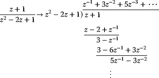
is a response that will have a value of 1 at the end of the first interval T, 3 at the second, 5 at the third and so on.
The idea of an impulse response arises from feeding a unit impulse input δ(t) to a system. In the z-domain, it is seen that the output values at the sampling instants arise as the coefficients of the original transfer function. For example, consider a unit impulse fed to an integrator, giving a finite impulse response which is a series of 1's:
In the case of integrating (or unstable/undamped) systems, one expects an infinite series of nonzero coefficients. However, for non-integrating, stable and damped systems, the coefficients arising from an impulse input become insignificant after a finite number of steps, and one describes this as a finite impulse response (FIR). An example would be the first-order system
where stability and damping require a > 0 and thus ![]() .
.
In Example 3.11, the focus was on the handling of actual signals, subjecting impulses to a zero-order hold to create continuous step functions, and so on. In practice, the concept is often used as a sort of shorthand to represent a sequence of data values. A forward shift operator q, or backward shift operator q−1, is used to shift a time sequence of values in the same way as z or z−1, without invoking the theoretical basis of z-transforms.
3.9.3.2 Use of z-Transforms to Find the System Response
The use of z-transforms here will focus on the time-shifting properties of z or z−1. One notes that
returns the value of x at a time T before the present. If a transport lag from inlet u to outlet x is exactly 3T, then one could write
Consider a linear system which is expressed as a set of first-order differential equations with constant coefficients:
As in Equation 3.152, the Laplace transform yields
The inversion will depend on the time functions in the input vector. A special case will be considered here where the inputs u(t) are held constant at their starting values u(0), so
Recall that the s-domain functions represent zero values up until time zero, so that the input being considered here is a step from zero in each input variable, at time zero. Then
It is useful to expand the inverse matrices of the second term using partial fractions, that is
where α and β are constant matrices.
so
Since ![]() is diagonal, and A is square,
is diagonal, and A is square,
Thus,
Taking the inverse Laplace transform
This result involves the state transition matrix ![]() , which is known as the matrix exponential, represented symbolically as
, which is known as the matrix exponential, represented symbolically as
It can be evaluated directly in mathematical programs such as MATLAB®, and has similar properties to a normal scalar exponential, for example
There is an obvious resemblance to the SISO case of Equation 3.110 and Table 3.3. The frame of reference so far has been 0 < t < ∞, but the integration can be used in the same way for successive intervals T as follows:
The form of this equation has a strong resemblance to the continuous system case (Equation 3.100). Here one defines similar matrices for the discrete system
so that
In terms of the time-shift operator z, this is
so
The transfer function matrix for this discrete linear state system is thus determined by
with
This transfer function is taking a series of input values at time intervals T and providing the output values at corresponding intervals T. It replaces the integration step of the continuous system in Equation 3.100 over each of these intervals, under the specific condition that the input values vary in a series of steps, remaining fixed at the initial value for each interval. It is quite clear that this formulation replaces the combination of zero-order hold and continuous system G(s) in Figure 3.33, and provides a general MIMO approach to the SISO example (Example 3.11). The successive multiplication of several transfer functions on this basis would imply that the intermediate values are sampled and held between each system. In practice, this is very much how intermediate values from various calculations are only updated periodically in a processing plant computer database.
Following the same treatment as in the s-domain (Section 3.9.2.2)
Again, the eigenvalues λi of A* are the roots of the characteristic equation
and will contribute factors (z − λ1), (z − λ2),…in the denominators of the partial fraction expansion of any response. Table 3.7 shows the importance of these denominators in determining the response. Each term in the adjoint matrix shown will also be a polynomial in z, so Equation 3.289 can be expressed as
where the matrices Ni group the coefficients of the relevant powers of z. This relationship is analogous to the s-domain expression (Equation 3.163). The equation may be divided by z successively until the highest power is z0. In this form, it provides an alternative recursive predictor for x based on past values of x and u. The transfer function is often expressed using a matrix of polynomial ratios. For this state system it is seen that the matrix G(z) has a common denominator for all elements (but these may all differ for a general input-output system).
3.9.3.3 Evaluation of the Matrix Exponential Terms
Equations 3.283 and 3.284 give the coefficient matrices of the discrete system
The matrix exponential ![]() is provided directly in environments such as MATLAB® (‘expm'), but it is worth noting that its Taylor expansion is
is provided directly in environments such as MATLAB® (‘expm'), but it is worth noting that its Taylor expansion is
since e0 = I. It follows then that
This latter result for B* is particularly useful when the matrix A is singular.
3.9.3.4 Shortcut Methods to Obtain Discrete Difference Equations
The procedure used in Section 3.9.3.2 to obtain an exact discrete equivalent of a continuous system with a piecewise-constant input has been laborious, though one notes that the matrix exponential is readily available in mathematical programs. Useful transfer functions are easily found in the s-domain, so several methods have been devised to convert these directly to approximate discrete equivalent equations. Noting that s represents a derivative, the following substitutions are used:
- Forward difference (implicit Euler):
(3.325)

- Backward difference (explicit Euler):
(3.326)

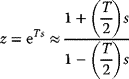
- sTustin (bilinear or trapezoidal):
(3.327)

Inverting the Tustin approximation,
which is the first-order Padé approximation, sometimes used in the s-domain to deal with transport lags in the quest for polynomial-ratio forms. The inverse form of these approximations (like Equation 3.328: z = fn(s)) is sometimes used for frequency analysis of discrete systems, by substitution of jω for s in the resulting equation, as discussed in Section 8.6.1.
3.9.3.5 Open-Loop Stability in the z-Domain
Equations 3.289–3.295 in the previous section examined the impact of the discrete system transfer function G(z) itself on the output x(z), regardless of the particular input u(z). The full-state representation is
and
So the characteristic equation for this open loop is
It is noted that the factors (z − λ1), (z − λ2),…will occur as denominators in the partial fraction expansion of any output x(z).
In Table 3.7, one needs to set λ = e−αT, and it is seen that
The possibility does exist that λ is complex:
that is
Thus, in the time domain, terms of the following form will occur in the system response:
The presence of a complex conjugate root λ will cause the imaginary values to disappear in the characteristic equation. Whether or not there is oscillation, there will be unbounded growth in the output if ln(a2 + b2) is positive (making α negative), meaning that all roots of the characteristic equation of a discrete system must lie within the unit circle for the system to be stable (Figure 3.34). This result is not surprising when it is recalled that z = esT, since it has been established in Section 3.9.2.3 that the real part of the solutions of the s-domain characteristic equation must all be negative for stability, that is to ensure that no bounded input can cause an unbounded output.

Figure 3.34 z-domain characteristic equation roots (stable: λ1, λ2, λ3; unstable: λ4, λ5, λ6, λ7).
As in the case of continuous systems (Section 3.9.2.3), discrete systems more generally can be represented in the input–output form
and again one expects the terms in matrix G′(z) to be ratios of polynomials in z, but here the denominators may all differ, giving more factors (see Section 7.8.1). For the same reason as above, the factors of these denominators, (z − ai), require |ai| < 1 for stability. The input–output form (Equation 3.345) is often represented as
where the backward shift operator q−1 replaces z−1. This reflects models based directly on data sequences, rather than implying any theoretical relationship to continuous systems.
3.9.4 Numerical Solution for System Response
From Equations 3.6–3.9, the general form of the system model based on physical principles is
for a given ![]() , where x is the vector of continuous states, w the discrete states, y the continuous and discrete ancillary variables, and u the continuous and discrete manipulated and disturbance variables. The vectors of functions f and g may be nonlinear, and may have logical conditions within them which change the behaviour depending on the other variables.
, where x is the vector of continuous states, w the discrete states, y the continuous and discrete ancillary variables, and u the continuous and discrete manipulated and disturbance variables. The vectors of functions f and g may be nonlinear, and may have logical conditions within them which change the behaviour depending on the other variables.
The examples in Sections 3.1, 3.2 and 3.3 considered systems which had some of these complications. An algorithmic ‘freehand' form of modelling was suggested that employed a simple Euler integration. This type of solution can be ‘improved' (faster, more accurate, less computation) if some restrictions are imposed. Some approaches are
- linear and logical (e.g. Bemporad and Morari, 1999);
- differential, algebraic and logical (e.g. Mao and Petzold, 2002);
- differential and algebraic (e.g. MATLAB®, Ascher and Petzold, 1998);
- stepwise re-linearisation and linear solution (e.g. Becerra, Roberts and Griffiths, 2001).
After developing a model, the process engineer's first task is to check how well the model represents the process, so that at least some basic tools are needed to integrate it. However, it is unwise to complicate the solution too early, as it is easy to lose sight of the basics and risk algebraic errors. So this discussion will restrict itself to some simple ideas concerning the integration of the system of first-order ODEs
for a given ![]() , which excludes discrete and ancillary variables. The solution will be based on past and present values of x and u, and can be expressed after time discretisation of Equation 3.352 in the general form
, which excludes discrete and ancillary variables. The solution will be based on past and present values of x and u, and can be expressed after time discretisation of Equation 3.352 in the general form
for given ![]() and
and ![]() .
.
If it possible to separate out xi+1 onto the left-hand side of Equation 3.353, it is said to be explicit, otherwise it is implicit.
3.9.4.1 Numerical Solution Using Explicit Forms
An explicit Euler integration formula for Equation 3.352, using a time step of T, is obtained as
The explicit Euler integration method is seen to use a single gradient vector evaluated at the start (or left) of the interval. The effects of this bias can be reduced by means of a smaller integration step T. However, it is worth noting another well-known explicit technique that seeks to eliminate this left-hand bias, the fourth-order Runge–Kutta method. In this technique, the estimates of the gradient are successively updated as new estimates are obtained of the change in x across the interval (Equations 3.361–3.364). It is seen that the final estimate (Equation 3.365) is based on a gradient that is more heavily weighted towards the centre of the interval.
A general observation regarding explicit methods is that the exclusion of xi+1 from the formulation leaves them prone to overshoot resulting in instability. MIMO systems of ODEs often have widely varying time constants (‘modes') in the equations, so that if a single time step is used, it might have to be very small to deal with this stiffness.
3.9.4.2 Numerical Solution Using Implicit Forms
An implicit form of stepwise integration would appear like Equation 3.353:
The equation might be written like this, but occasionally some manipulation allows extraction of xi+1. However, the general case will require an iterative solution for xi+1, for example using the Newton–Raphson method:
where ![]() is a Jacobian matrix obtained by differentiating each function in the h vector by each element in the xi+1 vector, and evaluating the result at the
is a Jacobian matrix obtained by differentiating each function in the h vector by each element in the xi+1 vector, and evaluating the result at the ![]() condition. Similarly,
condition. Similarly, ![]() represents the vector h evaluated with the estimate
represents the vector h evaluated with the estimate ![]() (and of course the earlier solutions xi, xi−1,…and ui,…, ui−m).
(and of course the earlier solutions xi, xi−1,…and ui,…, ui−m).
An implicit Euler integration for Equation 3.352, using a time step of T, is
However, it is noted that the gradient being used is now biased to the right of the time interval. Since one is already committed to an implicit solution, why not attempt an ‘average' value of the gradient using average values of the variables? Thus, a possibility is
3.9.5 Black Box Modelling
The open-loop modelling of the process discussed above has focused on mathematical descriptions of the physical phenomena occurring in the system. This type of modelling has the advantage that correction and adjustment of the model to match the process is based on meaningful parameters. In addition, the model operation can be extrapolated over new ranges with some confidence. Setting up such a mathematical description can, however, require a lot of skilled manpower, and there are cases where ‘black box' models, based mainly on input and output observations, have proved quite adequate for process optimisation and control. A brief review of some of the popular black box methods follows. The view taken here is that a large amount of historical process data is available (e.g. step test measurements), and can be used offline to develop the required models. A similar problem, in which this type of model is identified in real time, will be discussed in Section 6.5.
3.9.5.1 Step Response Models
As will be seen in Section 7.8.2, models based on measured process step responses have become very important as they form the basis of common controllers such as the dynamic matrix control algorithm. However, the model part of this model predictive control technique needs to be recognised as a useful open-loop modelling method in its own right.
Consider the two-input, two-output system in Figure 3.36 as being representative of MIMO systems in general. Because the observable outputs are not necessarily all of the states, or indeed the states at all, these will be represented by the vector y instead of x. With the system at steady state, each input is stepped in turn to obtain a matrix of step responses. For example, consider the effect of u1 on y1. The step of u1 from u1SS to u1SS + Δu1(0) at t = 0 produces y1 values at subsequent intervals T of y1SS + Δy1(1), y1SS + Δy1(2),…Normalising these with respect to the input step,
one obtains the unit step response function
Here q−1 is being used to represent a backward shift of one time interval, rather than z−1, as is conventional when none of the theoretical z-transform properties are intended. So far, a non-integrating system has been assumed, and the interval T and number of points N in each response have been chosen to both give good definition to the variations, and ensure that the final point is close to the new equilibrium of the system. In Equation 3.378, the final point has been extended indefinitely with a delayed unit step (see Table 3.7).
Figure 3.36 Step response measurement matrix for a MIMO system.
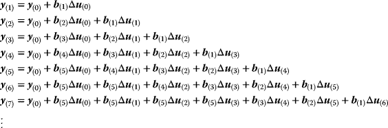
The important assumption one makes in step response modelling is that the system is linear. So if a system is initially at steady state y1(0), a positive or negative step of any size Δu1(0) at t = 0 must produce the following x1 output:
Notice that the product ![]() only gives the change in y1 from its initial value, so a step function is used to add back the offset at each future point in time. If there are now subsequent ‘moves' of u1 at the intervals T, that is
only gives the change in y1 from its initial value, so a step function is used to add back the offset at each future point in time. If there are now subsequent ‘moves' of u1 at the intervals T, that is
then the appropriate responses are just delayed in time before being summed:

Now include the effects of moves in u2, and treat y2 similarly to obtain
that is
Another way of viewing this is
where
Matching up the time-shift coefficients
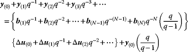
This is conveniently represented using a matrix of matrices and several vectors of vectors:
with

Note that the equations developed to this point rely on the system being at steady state at y(0) at t = 0. The matrix ![]() is referred to as the dynamic matrix, and will later form the basis of dynamic matrix control (Section 7.8.2). It is obvious that if there had been input moves Δu prior to the starting time t = 0, these would have an effect extending past t = 0, and would have to be included.
is referred to as the dynamic matrix, and will later form the basis of dynamic matrix control (Section 7.8.2). It is obvious that if there had been input moves Δu prior to the starting time t = 0, these would have an effect extending past t = 0, and would have to be included.
Up to this point only non-integrating systems have been considered, that is systems which reach a steady state within the N times represented in the dynamic matrix (with N = 5 in the preceding 2 × 2 example). Now consider a simple strategy for dealing with integrating systems. A possible coding of the final gradient of a response might be in terms of the last two points (N − 1 and N) of the step response (Figure 3.37). So the integrating gradient of y1 for a unit step input Δu1(0) is ![]() .
.
Figure 3.37 Integrating step response.
Then an appropriate delayed ramp function is included in b(z) in Equation 3.384 to obtain

The equivalent dynamic matrix for Equation 3.387 then becomes
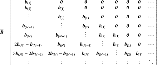
Equation 3.387, taken together with the possibility of Equations 3.389 and 3.390 for integrating systems, constitutes the important results of the step response modelling approach. One notes in Equation 3.388 that the output vector values correspond to the end of each interval, whilst the input vector moves are at the start of each interval. The response at the end of an interval T is independent of the input move at that same time, owing to the finite response time required, so the output vector starts at one interval later in time.
The step response modelling approach easily handles transport lag (dead time), since an arbitrary sequence of response values can be specified. In practice, several step response measurements should be done on a plant, to ensure that the features used in the model do not include random and temporary disturbances. Some degree of averaging and smoothing is necessary, and in some installations, a standard response such as first-order plus dead time may be fitted to the measurements for use in a controller. Many industries represent their dynamic matrix as an array of s-domain transfer functions, that is those functions that would convert each input step into the observed output responses.
As mentioned, a limitation of the method is that it assumes linearity. Model validity will thus be improved if the step responses are determined close to the normal operating point. One method used to handle severe process nonlinearity is to superimpose a separate nonlinear model, for example an artificial neural network (Example 3.17), just for the residual nonlinearity.
Another limitation to bear in mind is that the method does not explicitly recognise the relationships between variables in the same way as a mathematical model based on physical principles. For example, consider the two-tank flow system in Figure 3.38.

Figure 3.38 Step response modelling cannot find the equilibrium with both valves shut.
The separate step responses to each valve do not carry the information that if both valves shut, the levels must equilibrate. The nonlinearity of the level/flow relationship will cause the step response model to find two different tank levels at steady state, with both valves shut (assuming the step response measurements were not made at this state). Even if this relationship were linear, one would have to ensure that the initial output y(0) used to start the model represented an equilibrium to avoid this situation.
3.9.5.2 Regressed Dynamic Models
Historical plant measurements stored at intervals T constitute an input–output data set of the form

where u(i) is a vector of the input variables (MVs and DVs) at time iT and y(i) is a vector of the output variables (PVs or CVs) at time iT. Proper identification of the dynamic behaviour of this system will only be possible if the sampling interval T is not larger than about one-tenth of the shortest time constant in the system, that is one requires about 10 data points to define the shortest transient. A problem arising from too large a sampling interval is that of aliasing (Figure 3.39), where a higher frequency signal manifests at a lower frequency. Usually one is not concerned with frequency signals, but the same effect may cause misinterpretation of any signal.
Figure 3.39 Aliasing due to too large a sampling interval.
A form of model must initially be selected, requiring identification of the defining variables and the system order, plus an appropriate interval T for a discrete model.
Here p is a set of constant parameters used in the model. The determination of the model then consists in finding p which minimise some performance criterion, for example a least square deviation:
3.9.6 Modelling with Automata, Petri Nets and their Hybrids
Sometimes systems are too large and complex to be represented as a single monolithic set of equations and conditions, and it helps conceptually to divide them up into clear-cut entities which interact with each other according to well-defined rules. One approach is to use automata, or a particular form of these, the Petri net. These techniques originally grew around the idea of systems with a finite number of discrete states, but the methods were subsequently hybridised by the inclusion of continuous components. Along the way, a lot of useful theory and software has been developed, so if one is prepared to constrain one's approach to a problem to these established formalisms, one can take advantage of this background. The introductory discussion here will focus on how these approaches can be used to model concurrent systems which are linked by events.
An automaton is an entity for which a set of states and transitions are defined as in Figure 3.42. The initial state must be known in order to determine the outcome of a series of transitions. Conditions which must be satisfied before a transition can occur are called guards. Reconsider the tank problem of Figure 3.3, repeated in Figure 3.43, in terms of its possible states:
- 0: Level below H and disc intact.
- 1: Level above H and disc intact.
- 2: Level above H and disc burst.
- 3: Level below H and disc burst.
Figure 3.42 State and transition relationships for additive colours.
Figure 3.43 Tank with two restricted outflows and a bursting disc for automaton representation.
A hybrid automaton representing this system could be expressed as in Figure 3.44, where both the discrete states and continuous variable are handled simultaneously. Available treatments for such systems are somewhat restricted, for example timed automata with linear equations.

Figure 3.44 Hybrid automaton for tank in Figure 3.42, showing guards on transitions.
Petri nets similarly focus on states and transitions, using tokens to ensure that the conditions for a transition are met, including concurrency with other transitions. Since the original work by Carl Petri in 1962 (Petri, 1962), many permutations of this approach have been developed, including stochastic, timed, coloured, fluid and hybrid Petri nets. Initially, consider just the basic definitions:
- A Petri net is a bipartite directed graph consisting of two types of nodes: places and transitions.
- Each place represents a certain condition in the system.
- Each transition represents an event which could change the condition of the system.
- Input arcs connect places to transitions, and output arcs connect transitions to further places.
- Tokens are dots (or integers) associated with places. The presence of a token means that the condition has been satisfied.
- A transition fires when all of its input places have at least one token, and in so doing it removes one token (or more if specified) from each input place, and puts one token into each output place.
- The marking of the system is the distribution of tokens in its places.
- A marking is reachable from another marking if there exists a sequence of transition firings capable of taking the system from the original marking to the new marking.
- An arrow-headed arc arriving at a transition enables the transition. If it has a small empty circle instead of an arrowhead, it inhibits the transition (assuming a token is available).
The original Petri net framework as defined above is well suited to the calculational representation of event-based systems, such as the motor start/stop system of Figure 2.36, represented in Figure 3.45. In this example, the initial marking has the motor off and the start button (NO) pressed, so the next state will be ‘motor on' – the new marking will be a single token in the ‘motor on' place.

Figure 3.45 Petri net for motor power latching circuit.
Some extensions of these basic ideas include timing and delays which can be assigned to transitions (represented by a wider bar with a numeric indication of the delay period). Fixed firing rates can be used for continuous variables, guards can be placed on arcs and hybrid systems can include both discrete and continuous variable states. The drive towards hybrid representations has been fuelled by the usefulness of Petri nets in graphically representing biochemical reaction networks, for example for drug metabolism and interaction. These descriptions needed to include concentrations and reaction mass balances based on differential equations.
Figure 3.46 represents three levels of detail which might be used to represent a tank-filling operation using Petri nets. The version (a) only has the discrete states, and no information concerning the timing or intermediate values of the tank contents. Version (b) is a timed Petri net which makes use of a delay transition (wider black bar), which in an event-driven system will allow ‘time stamping' of the occurrence of the represented events. However, this form relies on constant flow rates, and complete knowledge of the states, for example it could not start with the tank partially filled.
Figure 3.46 Petri nets with three levels of detail for a tank-filling operation.
The hybrid version (c) shows the typical arrangement where the discrete network and continuous network function in parallel, with limited interconnection. Continuous places are shown as a double circle, and continuous transitions are shown as a double bar (empty narrow box). Associated with a continuous transition is a firing speed at which it automatically and continuously fires. The ‘tank being filled' transition in Figure 3.46 will be firing at a rate f, which is the volumetric rate delivered by the stock pump. So when it is enabled, a volume fΔt will be delivered from the stock to the tank over an interval Δt. Two loops cause this continuous transition to interact with the logical states. Firstly, the pump must be switched on, and secondly the receiving tank must not yet be full. On each firing, the ‘tank being filled' transition must be able to take a token from each of the two logical places, but it returns them immediately. As can be seen, the continuous ‘tank contents' place is able to supply a token to the ‘tank filled' transition through the V = Vmax guard, that is once the level V reaches Vmax. So at that point the ‘tank not full' token would be lost and filling would cease.
Figure 3.47 is a hybrid Petri net representation of the tank with two restricted outflows and a bursting disc in Figure 3.43. As in version (c) of Figure 3.46, the hybrid arrangement may seem cumbersome, and indeed the ability to treat it efficiently in the Petri net context is limited. An alternative is simply to use a discrete Petri net to supervise the execution of an associated set of equations – usually in differential and algebraic form (Champagnat et al., 1998). Much like the automaton in Figure 3.44 then, the place of the token in the discrete Petri net represents the particular set of equations which must be integrated as time moves on. The Petri net itself still provides the means to synchronise and ensure precedence of parallel calculations in a distributed system.

Figure 3.47 Hybrid Petri net for tank with two restricted outflows and a bursting disc in Figure 3.43.
3.9.7 Models Based on Fuzzy Logic
The principles of fuzzy logic were established by Lotfi Zadeh in 1965 (Zadeh, 1965). Whereas regression allows one to fit a model to a collection of measurement data, fuzzy logic allows the fitting of a model to human sentiment and experience, and to extract useful numerical estimates from this ill-defined information.
Fuzzy logic is based on fuzzy set theory. This allows for partial membership of a set, as opposed to the traditional bivalent view in which an element either did belong (membership = 1) or did not belong (membership = 0). For example, an ambient temperature range might be described by cold, mild or hot. Whether or not 15 °C is cold or mild is subjective, and it is likely to have partial membership of both these sets (say, based on the views of a large population). The total membership must add up to 1. Various functional forms can be devised to represent these sets, but the use of straight-line segments as in Figure 3.48 is common. Here it is seen that 15 °C has a membership (or ‘truth') of 0.5 for ‘cold' and 0.5 for ‘mild'.
Figure 3.48 Three fuzzy sets describing a temperature range.
So sets based on variable x have functional forms A(x), B(x) and so on, and operations defined as follows (Figure 3.49):
The variables considered in fuzzy modelling are not often dynamically related – usually the equivalent of an algebraic representation is being sought. However, in keeping with this text's emphasis on dynamic modelling, an illustrative example will be based on the tank with two restricted outflows and a bursting disc (Figure 3.43). By predicting the rate of change of level in the tank, the result will lend itself directly to dynamic modelling.
There is some similarity between the concepts of fuzzy modelling, and expert systems in general. An expert system is preloaded with a rule base based on ‘expert knowledge' in much the same way as the rules are constructed in fuzzy logic. However, there is generally no direct connection to numerical scales, with expert systems using an inference engine to navigate logical trees to obtain a conclusion of a discrete nature. The user input information can in cases be entirely preloaded, but because redundancy will occur with the narrowing of options as the search progresses, it is more efficient to enter data on demand.
3.10 Use of Random Variables in Modelling
The modelling discussed so far has been deterministic in nature, but one is often interested in stochastic (or random) behaviour. The area of robustness of control systems (Section 8.8) addresses the problem that the basis of model and controller development is usually some kind of simplistic statistical average, or perhaps even a single random sample. Then what if the real behaviour differs? In the open loop, to what extent should one expect the real output to differ from the model? In the closed loop, there can be serious implications for performance and stability.
Two issues are usually of interest: (a) the variation of input signals and disturbances and (b) the variation of the intrinsic system behaviour. Rather than embrace the fields of stochastic differential equations or even attempt to model the moments (mean, variance, etc.) of the outputs, one can learn a lot just by supplying the model with inputs and disturbances of a random characteristic nature, or varying the assumed model parameters in a random way.
Figure 3.52 shows two common probability density functions used to represent the range of values obtained in random sampling. Most natural processes produce samples which follow the Gaussian (or ‘normal') distribution (a). The (pseudo-) random numbers available on most computer systems, however, follow a top-hat distribution (b) over a range 0 < x < 1. In this range, one has uniformly f(x) = 1, since the cumulative probability up to x

must reach 1 for x = 1.
Figure 3.52 Gaussian (normal) and uniform (top-hat) probability density functions with mean µx and standard deviation σx.
According to the central limit theorem, the Gaussian distribution can be approximated by creating individual samples by summing n top-hat samples – the larger the value of n, the closer the approximation.
Consider the case where it is wished to use n samples from a {0, 1} uniform distribution to create a single random sample with a Gaussian distribution of mean µy and standard deviation σy. Firstly note that one requires
Since the samples z drawn from the {0, 1} distribution will have
each z sample must be transformed according to

before the n samples x are summed. Even with n as low as 4, a good approximation to the shape of the Gaussian distribution is obtained, though it should be clear that no y sample could ever occur outside the range
An alternative way to produce random normally distributed samples is through the cumulative probability function obtained for the Gaussian distribution as in Figure 3.53, after noting that
In practice, it is very unlikely that signal disturbances or model errors will vary in an uncorrelated way between sampling intervals – unless the sampling interval is large compared with the relevant time constants. So it is useful in simulation studies to prepare random variations of signals or model parameters which have a degree of autocorrelation. A simple way of doing this is by means of the single-exponential filter (Figure 3.54).
Figure 3.53 Inversion of a Gaussian cumulative probability function, with uniform {0, 1} samples as input, to get random Gaussian samples.
Figure 3.54 Single-exponential filter.
It is intended here to supply this filter with random samples x as input at the discrete time intervals. The filter will then produce a correlated random output y, making this a Markov process like Brownian motion. The input x will be unrelated samples, say from a Gaussian distribution as above. The output will also be distributed in the Gaussian sense, but will more importantly have autocorrelation, that is it will be correlated with itself across a time gap (Figure 3.55).
Figure 3.55 Typical autocorrelation function.
In the discrete system (Example 3.11), the z-domain transfer function for a first-order process with gain K, time constant τ and sampling interval T was

The transfer function for the single-exponential filter in Figure 3.54 is
Quite clearly
so the time constant τ of the single-exponential filter is
Appropriate choice of α and T then allows one to set the degree of variation of the signal y between sample points. One notes from Equation 3.437 and Figure 3.55 that the autocorrelation function for this filter is
Large α (near the maximum of 1) will give a slowly varying signal (T/τ small) and small α (near the minimum of 0) will give a fast-varying, almost uncorrelated signal (T/τ large).
In Example 3.19, a situation is represented in which a dynamic model of a process has been developed, and one wishes to provide a typically time-varying input signal, perhaps to check the performance of a controller, identifier or optimiser. Additionally, time-correlated random Gaussian errors are included in system parameters, representing model uncertainty and drift. This type of random perturbation of signals and parameters is referred to as Monte Carlo modelling, and it is often useful for revealing the effects of a large range of event combinations.
3.11 Modelling of Closed Loops
The focus so far has been on open-loop system modelling. In later chapters, controllers, identifiers and optimisers will be developed which one normally tests offline using a model of the process. Effectively, these algorithms just add extra equations to the overall system description, so there is nothing different to what has already been discussed. The most important aspect of closing a loop is to be aware of what can be manipulated and what cannot. In the open loop, MVs and DVs were accessible to excite a system. In the closed loop, some or all MVs will be taken over by the algorithm. Instead, higher level variables can now be set as input, such as setpoints and constraints (Figure 3.57).
Figure 3.57 Net inputs and outputs for open-loop and closed-loop modelling.
References
- Ascher, U.M. and Petzold, L.R. (1998) Computer Methods for Ordinary Differential Equations and Differential–Algebraic Equations, SIAM, Philadelphia, PA.
- Becerra, V.M., Roberts, P.D. and Griffiths, G.W. (2001) Applying the extended Kalman filter to systems described by nonlinear differential–algebraic equations. Control Engineering Practice, 9 (3), 267–281.
- Bemporad, A. and Morari, M. (1999) Control of systems integrating logic, dynamics and constraints. Automatica, 35, 407–427.
- Champagnat, R., Esteban, P., Pingaud, H. and Valette, R. (1998) Petri net based modelling of hybrid systems. Computers in Industry, 36, 139–146.
- Mao, G. and Petzold, L.R. (2002) Efficient integration over discontinuities for differential–algebraic systems. Computers & Mathematics with Applications, 43 (1–2), 65–79.
- Petri, C.A. (1962) Kommunikation mit Automaten. Ph.D. thesis, Darmstadt University of Technology.
- Zadeh, L.A. (1965) Fuzzy sets. Information and Control, 8, 338–353.