
8
Stability and Quality of Control
8.1 Introduction
Control theory has until recently been taught in a way that did not distinguish much between the fields of application, whether those be missiles, aircraft, power systems or chemical processes. The advent of the digital computer has however opened up a vast range of new applications, which have perceptibly moved the emphasis away from the types of things that the classical analysis methods handled. This is particularly the case in the processing industries where the control engineer has a new focus on advanced process control (APC), model predictive control (MPC) and real time optimisation (RTO). Of course, issues of loop stability and controller performance are still important, but in the process industries these are seldom investigated by classical methods such as frequency response and root locus. The new computer-based work is exclusively in the time domain. In comparison with other fields, the frequencies to be dealt with are very low, often arising from the control loops themselves! ‘Good’ initial settings for controllers may be estimated theoretically before start-up, but the fine-tuning tends to be based on trial-and-error experience. The signs of instability are early detected as undesirable process fluctuations, and tuned out. In this largely ‘regulation’ mode, no one is pushing the limits at the edge of instability. One reason for this approach is that the processes are nonlinear and variable, and seldom match a model tightly, as might be the case in mechanical and electrical systems. So there is little point in pushing the control performance close to the limits of a model.
Despite this gloomy view of the relevance of many classical ideas, they are nevertheless important because they underlie the perception and language of the new applications. This has a parallel in the way modern digital control in a DCS or SCADA is represented as a mimic of the old analogue controllers. Nowadays one might say that there is a ‘badly damped pole’ in the closed-loop control of a distillation column. One is thinking how different terms in a characteristic equation (arising from submodels) can contribute uniquely different behaviours to a system – in this case with a slowly decaying oscillation. One is imagining a position on the complex plane, but there is no way that one is about to embark on a calculation in complex algebra to present to the boss!
In Figure 8.1, a potentially multivariable system is represented in open loop and in closed loop in a classical sense. In terms of modern controllers, this is already a restriction, as the controller often does not work exclusively on the deviation from setpoint – more information may be required such as absolute and previous values. The ‘real output’ is an abstract construct because there is no way of knowing precisely what it is, having to work remotely through sensors, whether they entail human sensing (e.g. vision) or instrument sensing. For example, any practical sensor will have a response lag. So, the idea of an ‘actual output’ can be bypassed and loops dealt with as unity feedback. That is, from a ‘plant’ point of view, the knowledge of what the output is is indistinguishable from the available measurement.

Figure 8.1 Classical views of open-loop and closed-loop systems.
Figure 8.1 also shows the two possible routes used for the entry of disturbances into the system – something that becomes important in the development or testing of algorithms for disturbance (load) rejection – the main area of concern in the process industries. The disturbance w is equivalent to a random disturbance of the control action – such as a jittery deviation from the set valve position. The disturbance d is equivalent to deviations in the ‘actual’ variable, such as liquid surface ripples in level control.
In Section 3.9.2, methods were developed to represent the dynamic alteration of signals using Laplace-domain transfer functions G(s). A series of dynamic elements acting on a signal could be represented as a multiplication of all of the transfer functions.
The classical open-loop transfer function is
Ignoring the disturbances in Figure 8.1
So, the closed-loop transfer function is
which is represented in SISO systems as
The view taken above is that of servo control, which is to do with the tracking of setpoint variations as in vehicle guidance. In the process industries, regulator control is far more important, so one is interested in the behaviour from, say, disturbance d to b. Ideally one would like to see this being a zero transfer function! Recalling the linearity assumptions in Section 3.9.2, where the variations were taken as deviations from an operating point, regulator mode can be represented as r(t) = 0:
A system may be open-loop unstable (e.g. an exothermic reactor) – it will be seen as in Section 3.9.2.3 that this is determined by denominator terms in GO(s). In the closed loop (Equation 8.5 or 8.12), the stability behaviour will be seen to be determined by the ‘denominator’ term ![]() . The interest in stability is not simply whether a system is stable or unstable. Usually as one tries to improve the performance of a controller (e.g. higher gain), one approaches more closely an unstable situation. So, it is useful to have a measure of how close one is to instability as a design criterion.
. The interest in stability is not simply whether a system is stable or unstable. Usually as one tries to improve the performance of a controller (e.g. higher gain), one approaches more closely an unstable situation. So, it is useful to have a measure of how close one is to instability as a design criterion.
8.2 View of a Continuous SISO System in the s-Domain
8.2.1 Transfer Functions, the Characteristic Equation and Stability
8.2.1.1 Open-Loop Transfer Functions
In Section 3.9.2.1, it was found that a continuous linear SISO open-loop system could be represented by
For physically realisable systems, one requires m ≤ n. Taking the Laplace transform yielded the transfer function
The numerator NO(s) and denominator DO(s) polynomials could be factored to yield
where K = bm/an. The zi are the ‘zeros’ of the open loop, because s → zi causes GO(s) → 0. The pi are the ‘poles’ of the system, because s → pi causes GO(s) → ∞. The characteristic equation of the system in Equation 8.14 arises from setting the denominator to zero. Obviously the poles are the roots of the characteristic equation.
Characteristic equation of the open loop:
Any pole or zero may be complex. However, it is easily shown that if a complex pole exists, its complex conjugate will also exist as a pole, and likewise for the zeros. The biggest hurdle in getting a linear system to this form would be the presence of dead time, which was found in Section 3.9.2.1 to have instead a transfer function ![]() . In ‘frequency-domain’ analysis, this can be dealt with explicitly in the form
. In ‘frequency-domain’ analysis, this can be dealt with explicitly in the form
Only where one specifically needs to represent the system entirely in terms of poles and zeros (e.g. root locus), it is necessary to substitute an approximation of e−τs in the form of a ratio of two polynomials, for example
first-order Padé approximation:
second-order Padé approximation:

which will revert the system to the form shown in Equation 8.14 or 8.16.
8.2.1.2 Angles and Magnitutes of s and GO(s)
Consider a general transfer function of the form shown in Equation 8.18. The poles and zeros may be complex, so for a particular choice of s on the complex plane, the vectors represented by the algebraic factors are merely complex numbers with angles and magnitudes as in Figure 8.2.

Figure 8.2 Complex vectors representing transfer-function factors.
A complex number s = a + jb has an angle and a magnitude as follows:
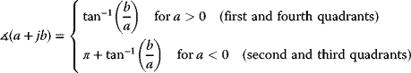
There is a polar notation in which the number is represented as
Recalling that
and
one writes equally
Applying this in Equation 8.18 then yields, for example
so that
This has allowed for the possibility that K < 0 (in which case ![]() ).
).
8.2.1.3 Open-Loop and Closed-Loop Stability
In Section 3.9.2.1, it was found that the open-loop denominator factors in Equation 8.16 would occur in the partial fraction expansion of the system output regardless of the input:
Here, the possibility of a repeated pole p1 is included. The extra α, β,…terms arise from the denominator of the input function U(s).
Now consider a particular root pi of the characteristic equation which may appear n times (i.e. an nth order root). Allow for the possibility that pi is complex, that is,
Because the complex conjugate pole must also exist, the following pair of terms will exist in the partial fraction expansion for a root repeated n times
From Table 3.5 the inversion to the time domain is given by
Noting Equation 8.31 for repeated poles, similar terms will coexist for n values down to 1, where 0!=1. Regardless of the order of a pole, or whether it is complex, the process GO(s) itself will contribute a series of terms in the output which have a factor ![]() , where ai is the real part of pole i of GO(s). This factor will start at unity for t = 0, and with time will increase to infinity if ai > 0, and will decrease to zero if ai < 0. Unbounded growth (ai > 0) for any one pole i determines an unstable system. If all poles i have ai < 0, (thus causing progressive attenuation of any disturbance), the system is said to be stable.
, where ai is the real part of pole i of GO(s). This factor will start at unity for t = 0, and with time will increase to infinity if ai > 0, and will decrease to zero if ai < 0. Unbounded growth (ai > 0) for any one pole i determines an unstable system. If all poles i have ai < 0, (thus causing progressive attenuation of any disturbance), the system is said to be stable.
These ideas about stability have been developed around a consideration of a nominal ‘open-loop’ transfer function GO(s). Any system that can be got into the form of Equation 8.16 can be considered in the same way, whether it be open loop or closed loop. However, the open-loop stability was first considered because classical theories draw many inferences about the closed loop from the open loop. For this to be possible, the open loop must include every element around the loop, as in the e → b case at the top of Figure 8.1. From Equation 8.7,

This is just a new equation of the form shown in Equation 8.14 having the characteristic equation
which will have n roots because n ≥ m. More succinctly, the closed-loop characteristic equation is written
A review of Equation 8.34 gives useful insight into the contribution of the poles of any process G(s) (open loop or closed loop) to its output behaviour. A time constant is identified with each term according to
The further the pole lies into the negative real complex half-plane, the shorter the time constant and the faster the response. As the damping factor ζ of a pole decreases, it contributes increasing oscillation which takes longer to attenuate (Figure 8.3). In Example 3.9 in Section 3.9.2.2, it was seen how ζ and τ arose in the definition of a standard second-order system – that is ![]() . (Clearly the ai and bi of pole i differ from the a's and b's in Equation 8.36).
. (Clearly the ai and bi of pole i differ from the a's and b's in Equation 8.36).

Figure 8.3 Behaviour of terms in the output as dependent on associated poles of the system.
8.2.1.4 Open-Loop and Closed-Loop Steady-State Gain
Whilst considering the open-loop and closed-loop transfer functions, it is opportune to introduce a useful property based on the final value theorem:
For a unit step input
Thus the steady-state gain of a system is got by setting s → 0 in its transfer function. (Later it will be seen that this is just the gain at zero frequency – i.e. steady state). Considering the forms shown in Equations 8.14 and 8.18 of G0(s), the open-loop steady-state gain is:
or

so the closed-loop steady-state gain is:
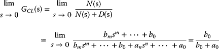
or similarly

8.2.1.5 Root Locus Analysis of Closed-Loop Stability
In Section 4.2, some basic SISO controllers were considered:
From Equation 8.2
with the controller gain now explicitly factored out of ![]() . The closed-loop characteristic Equation 8.37 is thus
. The closed-loop characteristic Equation 8.37 is thus
For the root locus analysis, one must start with the factored form of Equation 8.16, invoking approximations such as Equations 8.19 and 8.20 in the event of dead time. So, the closed-loop characteristic equation is
which will have n roots since n ≥ m.
Note: The roots loci of a system are the paths traced out by its closed-loop poles on the complex plane as the system gain increases from 0 to ∞.
The root locus plot is thus a useful aid to understand the effect of increasing controller gain on the closed-loop performance.
The loci of the n roots will start at the open-loop poles (for KC = 0), and as KC → ∞, m of these will end at the open-loop zeros, with the remaining n-m loci ‘heading for infinity’ (‘large’ s). This is what one would expect if Equation 8.51 is to ‘balance’. Certainly, where n > m, ‘large’ s would allow the s terms in the denominator to dominate the magnitude, as required to balance the large KC in the numerator.
Of course, one could generate the root locus plot automatically by stepping KC in small increments and using a polynomial equation solver on each step to obtain the new pole positions. However, the main features of the plot can be sketched out by inspection of the open-loop transfer function. The procedure for this can provide useful insight to the closed-loop behaviour. For the standard case of negative feedback (![]() ), one applies the following rules:
), one applies the following rules:
- Factorise the numerator and denominator of the open-loop transfer function, and write down the closed-loop characteristic equation in the form shown in Equation 8.51. On the Im/Re complex plane, mark the n open-loop poles with ‘×’ and the m open-loop zeros with ‘O.’ Bear in mind that these may be multiple-ordered - that is more than one on the same location.
The loci will follow paths traced out by positively charged particles in an electrostatic field where the ×'s are positive and the O's are negative. The positively charged particles must be released at the ×'s (but at which 360° position around the ‘edge’ of an × may need further clarification – see (5) below).
Because the loci represent the closed-loop poles, if any part of a locus is complex, a mirror-image complex conjugate part must exit – that is the loci must be symmetrical about the real axis (so that associated factors in the characteristic equation leave real coefficients when multiplied).
- The real axis will be part of the root locus if there is an odd number of ×'s plus O's to the right. Where two real ×'s or two real O's are connected together in this way, there has to be a break-out point or a break-in point, respectively. The leaving or entering loci do so at right angles to the real axis. The points are determined by solution of
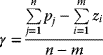
- m of the loci will proceed from ×'s to O's, and the remaining n-m will move outwards along asymptotes which diverge at equally spaced angles θk from a centre of gravity γ as follows:
(8.54)

- The q loci departing from a qth-ordered pole pa do so at the following angles leaving the ×:
(8.55)

The v loci approaching a vth-ordered zero zb do so at the following angles entering the O:

The proofs of these attributes are given by Coughanowr and Koppel (1965). Apart from direct algebraic solution of the characteristic equation, points on the roots loci can also be fixed by applying the angle criterion and the magnitude criterion to the closed-loop characteristic Equation 8.51, using the results of Section 8.2.1.2:
where k is an as yet unknown integer, and if ![]() , one obtains:
, one obtains:
angle criterion:
magnitude criterion:
The correct odd number of π's in Equation 8.57 is not clear until one is in the vicinity of the solution. Typically s must comply with an additional constraint such as a damping ratio line or magnitude circle which intersects the root locus. This intersection on a rough root locus plot provides a good starting guess of s which is then refined iteratively to comply with the angle criterion shown in Equation 8.58.
The method discussed above for generating the main features of the root locus plot apply to the standard case of negative feedback – that is, ![]() in the closed-loop characteristic Equation 8.51 is positive (Figure 8.5). There are situations in which it becomes negative (or a better way of thinking about it is that the ‘−1’ on the right-hand side becomes ‘+1.’ This will obviously change all of the angle references from ‘(2k + 1)π’ to ‘2kπ.’ There is a similar construction procedure based on this scenario that must be referenced in that case. An example of this occurrence is where a first-order Padé approximation (Equation 8.19) has been used for dead-time lag:
in the closed-loop characteristic Equation 8.51 is positive (Figure 8.5). There are situations in which it becomes negative (or a better way of thinking about it is that the ‘−1’ on the right-hand side becomes ‘+1.’ This will obviously change all of the angle references from ‘(2k + 1)π’ to ‘2kπ.’ There is a similar construction procedure based on this scenario that must be referenced in that case. An example of this occurrence is where a first-order Padé approximation (Equation 8.19) has been used for dead-time lag:

which apart from contributing the negative, is also seen to place an open-loop zero in the right-hand complex plane. Certainly, as KC increases, the closed-loop root locus approaching that zero will eventually cause instability.

Figure 8.5 Root locus plot for Example 8.2: Example 8.1 extended with an extra pole.
This case where ![]() in Equation 8.51 is termed the complementary case, and can be thought of as positive feedback. It is worthwhile noting how the rules change:
in Equation 8.51 is termed the complementary case, and can be thought of as positive feedback. It is worthwhile noting how the rules change:
- No change
- The real axis will be part of the root locus if there is an even number (including zero) of ×'s plus O's to the right. The entry and exit points are determined by Equation 8.52 as before
- The centre of gravity γ is determined by Equation 8.53 as before, but now the asymptotes radiate outwards at angles
(8.94)

- The q angles of departure from a qth-ordered pole pa become
(8.95)

and the v angles of approach to a vth-ordered zero zb become
(8.96)
With
 negative in Equation 8.51, the magnitude criterion shown in Equation 8.59 remains the same, but the angle criterion shown in Equation 8.58 obviously becomes(8.97)
that is
(8.98)
where k is an as yet unknown integer.
8.3 View of a Continuous MIMO System in the s-Domain
From Equation 8.6 the closed-loop transfer function is
with
As an example, consider a process determined by

Usually, there is no interaction between measurement devices so one might have

A properly compensating MIMO controller would have off-diagonal terms to handle the interactions, but in a typical multiple-SISO industrial control set-up, interactions are ignored and individual PI controllers might be specified as

So, in this case

Since ![]() , from Equation 8.99 the characteristic equation of the closed-loop MIMO system is
, from Equation 8.99 the characteristic equation of the closed-loop MIMO system is
so in this example the poles of the closed loop are obtained by solving

Without the dead-time delays (or if they are approximated as in Equation 8.19 or 8.20), this just requires a polynomial solution, which will give a number of pole positions on the complex s-plane for a particular choice of KC1 and KC2. The same principles obviously apply as in the SISO view of Section 8.1, except now the 0 < KC1 < ∞ root loci will vary for each choice of the KC2 value, and vice-versa.
8.4 View of Continuous SISO and MIMO Systems in Linear State Space
The approach will be developed for a MIMO system, but the same relationships apply for a SISO system. Referring to the closed-loop system in Figure 8.1, and ignoring disturbances, the continuous linear representation of the process in the state space is
Ignoring the nicety that b is not y, consider that the output of interest y is the same as the feedback signal so the error is
For argument sake, consider every element in the ‘controller matrix’ to be potentially PID, for example, in a 2-input, 2-output system,
Differentiating
with
and
Differentiating Equation 8.107 and substituting to close the loop
Using Equation 8.109 then one obtains

Representing the forcing input from the setpoint as F, the form is
where the stability is seen to be determined by the homogeneous part, by taking the Laplace transform
As seen in Example 3.9, the characteristic equation of this system is
of which the solutions are clearly the eigenvalues of H. As noted in Section 9.2.2.2, these must lie in the left-hand complex plane if the system (in this case the closed loop) is to be stable. If any eigenvalue of
has a positive real part, this closed loop will be unstable. In this example, one can extract the reduced case of proportional state feedback, where N = 0 and D = 0. Equation 8.117 reduces to
So, here the KCij values in the P matrix must be chosen in such a way that the eigenvalues of ![]() lie in suitably damped positions in the left-hand complex plane. Of course, the controller need not have the particular form of Equations 8.110 and 8.111, but the same considerations apply. A number of pole placement design techniques are available in the literature – see for example Sections 7.6.1 and 7.6.3.
lie in suitably damped positions in the left-hand complex plane. Of course, the controller need not have the particular form of Equations 8.110 and 8.111, but the same considerations apply. A number of pole placement design techniques are available in the literature – see for example Sections 7.6.1 and 7.6.3.
8.5 View of Discrete Linear SISO and MIMO Systems
Again, the MIMO system is treated as the general case. In Sections 7.5 and 7.8, discrete MIMO models were encountered in the format
or
with constant matrices Ni and Di determining
Where a model arose from input–output data (e.g. step responses) ![]() could be made scalar, as in Section 7.8.1. If it arose from state-space modelling, Equation 8.129 would have a state recursive form determined by
could be made scalar, as in Section 7.8.1. If it arose from state-space modelling, Equation 8.129 would have a state recursive form determined by ![]() and
and ![]() .
.
A MIMO controller ![]() will also have this form, for example, arising from a Tustin approximation as in Section 4.2.3, and likewise the measurement dynamics
will also have this form, for example, arising from a Tustin approximation as in Section 4.2.3, and likewise the measurement dynamics ![]() . Taking care with the order in which the signals are processed, the open-loop transfer function is
. Taking care with the order in which the signals are processed, the open-loop transfer function is
which will again have elements which are ratios of polynomials in z. In Figure 8.1, the closed-loop behaviour is determined by
Since ![]() , the characteristic equation determining the closed-loop poles is thus
, the characteristic equation determining the closed-loop poles is thus
Bearing in mind that for sampling interval T,
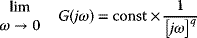
one notes that for stability Re(s) = a must be negative, so the roots of Equation 8.132 must lie within the unit circle on the complex plane (![]() ). In Figure 7.11, one notes that b determines the angular deviation from zero of z on the complex plane. The damping ratio is
). In Figure 7.11, one notes that b determines the angular deviation from zero of z on the complex plane. The damping ratio is ![]() , so it will increase as a pole z approaches the origin but will decrease as the angle of z increases.
, so it will increase as a pole z approaches the origin but will decrease as the angle of z increases.
8.6 Frequency Response
So far a view of open-loop and closed-loop stability has been developed around the location of poles on the complex plane. These poles were the solution of the characteristic equation (denominator = 0), the importance of which arises from the contribution of the roots to output responses, as becomes evident through a partial fraction expansion. Now an alternative view will be developed based on frequency, which offers new measures of relative stability, and has the advantage that it handles dead-time precisely. Noting the similarity of the Laplace transform
to the Fourier transform (Section 6.1.2), one expects s to have frequency units (time−1). Indeed, a simple substitution of jω for s (where ω is frequency in radians/time) will be seen to provide important information about the frequency response, that is the attenuation and phase lag of frequency signals passing through a system.
8.6.1 Frequency Response from G(jω)
Consider a linear SISO system subjected to a steady frequency signal
as in Figure 8.6. According to the condition of stationarity (Section 3.6), the output ultimately becomes a steady oscillation at the same frequency, that is,
where ϕ is the phase angle. Recalling the identity
one can write
As in Equation 3.129, consider a linear system with constant coefficients which can be represented by
Substituting u and x using Equations 8.147 and 8.148 obtain

Noting that ![]() , and that multiplication by
, and that multiplication by ![]() has the results
has the results
then Equation 8.150 yields

The variable t only occurs in ![]() in the first term on each side, and not the f1 and f2 terms. Hence, matching the remaining coefficients one has
in the first term on each side, and not the f1 and f2 terms. Hence, matching the remaining coefficients one has
Clearly then, at least for this polynomial ratio form of G(s), a steady oscillation passing through the system has a frequency response which is related to the input by
Actually, a dead-time factor ![]() can be included directly by the substitution s = jω, bearing in mind that
can be included directly by the substitution s = jω, bearing in mind that
and
Factorising the polynomials in Equation 8.156 (see Equation 3.133), an alternative view is
so that
Let
Obviously
that is

Figure 8.6 Steady frequency signal applied to a linear system G(s).
8.6.2 Closed-Loop Stability Criterion in the Frequency Domain
In the root locus analysis of closed-loop stability in Section 8.2.1.5, conclusions were drawn from inspection of the open-loop transfer function in the form of the closed-loop characteristic Equation 8.51. The frequency response methods are a bit like this because they too focus on the frequency response of the open loop in order to infer things about the closed loop. Of course, this open loop has to include every element as the signal passes around the loop (classical open loop in Figure 8.1), including the controller itself.
The argument for closed-loop stability in the frequency domain is illustrated in Figure 8.7. Usually (but not always) the phase lag (−ϕ) increases and the amplitude ratio (RAO) decreases as the frequency increases. A few systems (e.g. first order) cannot achieve phase lags as large as π, but for those that do, the particular frequency at which this happens is called the crossover frequency (ωCO). If this has been found, and an oscillation of this frequency is fed into the open loop (via the setpoint) as on the left of Figure 8.7, a situation arises where the feedback signal b has the same frequency but is inverted in comparison to e, and has a fixed greater or lesser amplitude, depending on whether RAO(ωCO) is greater than unity or less. Now say that two things are done instantly and simultaneously – the setpoint r is set to zero and the loop is closed. In the case where RAO(ωCO) = 1 there will be no change, because the feedback signal b is the exact inverse of e and it is inverted again at the comparator to replace the setpoint. It is intuitively obvious, though, that if RAO(ωCO) < 1 the oscillation will shrink (stable) and if RAO(ωCO) > 1 the oscillation will expand (unstable). The frequency domain stability criterion could thus be stated:

Figure 8.7 Illustration of frequency response stability criterion (RAO < 1 when ϕ = −π).
The situation that has been described might appear rather fortuitous – what if the signals are never in the frequency range that determines RAO > 1 and/or ϕ < −π ? The problem is that a typical disturbance like an impulse or step is constructed (in Fourier terms) from an infinite range of frequency signals, and the smallest signal with the correct frequency (ωCO) will continue to amplify itself indefinitely in the closed loop.
By measuring or calculating how close the open loop is to having a gain (amplitude ratio) of unity at the crossover frequency, or vice versa how close the phase angle is to −π when the gain is unity, one is able to obtain a measure of relative stability for the closed loop:
The condition at which the closed loop is on the verge of instability thus implies that simultaneously GM = 1 and PM = 0. These measures are usually presented in the units of decibels and degrees
To summarize the stability relationship:
| closed-loop stable | GM > 1 (GM > 0 db) | PM > 0° |
| closed loop on the verge of instability | GM = 1 (GM = 0 db) | PM = 0° |
| closed-loop unstable | GM < 1 (GM < 0 db) | PM < 0° |
Typical choices are GM = 9 db or PM = 40°. It would be coincidental if these were simultaneously met, and indeed, the PM sometimes cannot be calculated, viz. in the case where RAO never rises as high as unity. The maximum lags of first- and second-order systems are 90° and 180°, respectively, at very high frequency, so these will not have a crossover frequency, and indeed cannot become unstable if the loop is closed around them.
8.6.3 Bode Plot
The Bode plot consists of two sets of axes, one showing the variation of RA(ω) with ω, and the other the phase angle ϕ (ω) with ω. The abscissa ω in both plots is on a logarithmic scale, as well as the RA ordinate (usually in db). The ϕ ordinate is a linear scale. In Example 8.4 it was shown how the full response to a frequency signal (including the initial transient) could be calculated. In the limit as t → ∞ the same result is obtained for the steady-state response based on G(jω). So, there are two ways to arrive at a Bode plot based on the s-domain transfer function of the process. It is, however, more likely that this frequency response will simply be measured. Comparison of steady input and output oscillations over a range of frequencies as in Figure 8.6 provides the necessary data. Though the process itself might be measured, the proposed controller (e.g. PI) might only be known in the GC(s) form, in which case the two separate frequency responses are simply ‘added’ on the Bode plot to predict the open-loop frequency response, and hence the closed-loop stability (Figure 8.8). As in Equations 8.169 and 8.170, the phase angles are added, but the multiplication of magnitudes is of course equivalent to adding their logarithms.

Figure 8.8 Construction of Bode plot to achieve a desired gain margin in Example 8.5. (‘Measured’ GP was based on a second-order system with K = 10−3, τ = 0.2, ζ = 0.3.)
As in the case of root locus (Section 8.2.1.5), the main features of Bode plots can be sketched by inspection. This does not have great practical importance, but the ideas are again an aid to the understanding of system dynamics. Consider a general system in the factored form of Equation 8.163:
Recall that the frequency response if obtained by the substitution s → jω.
One can make the following observations:
-
(8.207)

which gives a constant RA asymptote as ω → 0, provided no poles are zero. As ω → 0, the phase angle ϕ will be either 0 or π depending on the sign of the expression.
- If q of the poles are zero,
(8.208)
which gives an RA asymptote of slope −q on a log–log plot, with RA increasing to ∞ as ω → 0. The phase angle in this limit asymptotes to −q × π/2 (shifted by π if const is negative).
-
(8.209)

so
 which is an asymptote of slope m–n on a log–log plot as ω → ∞. For physically realizable systems, m < n so the slope is negative and
  . As ω → ∞, the phase angle ϕ will approach
  .
.
8.6.4 Nyquist Plot
Whereas the Bode plot uses two sets of Cartesian axes to express the dependences of RA and ϕ on the frequency ω, the Nyquist plot, which is similarly plotted for the open loop, is rather a single polar plot of the magnitude RA at the corresponding angle ϕ, as ω varies. Unless the ω values are explicitly marked on this curve, one loses information about the frequency dependence. However, this account jumps ahead. One needs to start by considering the Nyquist stability criterion which is based on the Nyquist contour. It will be seen that the usual Nyquist plot only represents part of the Nyquist contour (where s = jω, 0 < ω < + ∞), but the stability of a loop closed around the plotted transfer function can nevertheless be inferred from such an open-loop plot.
Start by considering the factored form 8.163 of the open-loop transfer function
For an arbitrary choice of point s on the complex plane, a single factor like (s-zi) represents a vector pointing from zi to s as in Figure 8.9. Now let the point s move along a path that encircles zi in a positive angular direction (anti-clockwise). The angle θi of (s-zi) will be seen to increase through a net +2π. If zi had been outside of the chosen path (or ‘contour’), the angle would have oscillated up and down, back to its original value, but completing a zero net rotation. One net positive rotation of (s-zi) will manifest itself as one net positive rotation of G(s) about its origin, according to Equation 8.170. A positive encirclement of a pi in the expression 8.210 will conversely contribute one net negative rotation to G(s).
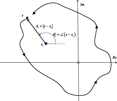
Figure 8.9 Variation of the angle of (s-zi) as s encircles zi.
For reasons that will become clearer later, the above phenomenon will now be used to detect the presence of open-loop zero's in the right-hand s-plane, without having to factorise the numerator polynomial as in Equation 8.210. Because the Nyquist contour has to encircle this entire half-plane, it is defined as in Figure 8.10 – that is a semicircle with infinite radius covering the positive real half-plane. Proceeding around the Nyquist contour ABCDEFA one obtains the corresponding trace on the Nyquist plot. The particular plot shown in Figure 8.10 has neither zeros nor poles with positive real parts, so the net rotation about the point G = (0 + j0) is zero.
![Figure depicting the mapping of Nyquist contour [s] into Nyquist plot [G(s)].](http://images-20200215.ebookreading.net/20/1/1/9783527341191/9783527341191__applied-process-control__9783527341191__images__c08__n8f010.gif)
Figure 8.10 Mapping of Nyquist contour [s] into Nyquist plot [G(s)].
It is noted that the part of the plot corresponding to DEFA is the complex conjugate of the first half ABCD. Moreover, for physically realizable systems, m < n, so the part corresponding to AB disappears at the G-plane origin. Finally, the part corresponding to CD is ‘off the G plot.’ The upshot of this is that in practice only the BC part is plotted (but one needs to bear in mind what the invisible parts are doing so that rotations can be counted). Thus, as already hinted, the Nyquist plot is simply a polar representation of the frequency response G(jω), with the positive angular direction determined by ω proceeding from +∞ down to 0. Some typical Nyquist plots are shown in Figure 8.11.
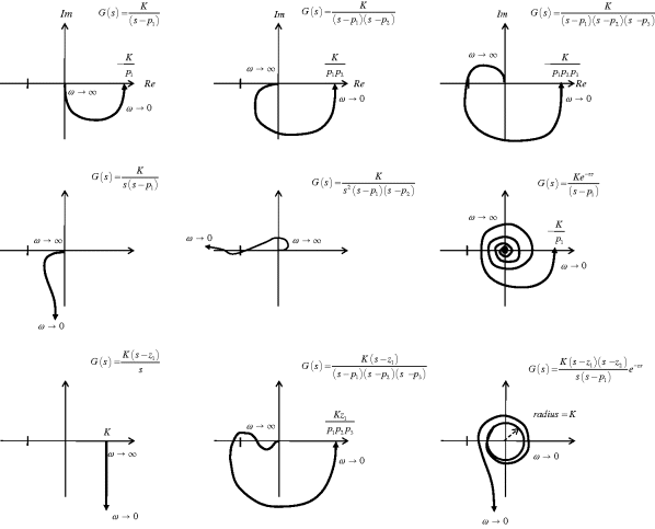
Figure 8.11 Examples of Nyquist plots.
Now the usefulness of the Nyquist plot, representing an open-loop frequency response, for determining closed-loop stability, will be explained. Firstly, insist that only open-loop stable systems will be considered. That means that not one of the pi in Equation 8.210 is lying within the Nyquist contour, and therefore these poles cannot contribute any net rotations of G(s) around its origin as s follows the contour. (For poles these would be in a negative angular direction). Consider a new transfer function
This has the same poles as G(s), so the number of positive rotations of G'(s) of its own origin must represent exactly the number of zeros of G'(s) which lie in the right-hand s-plane. In practice, one does not draw a new plot for G'(s), but rather just ‘imagines’ a new coordinate system with its origin at (−1 + j0) on the G(s) plot (Figure 8.12).

Figure 8.12 Imagined shift of origin when looking for ‘encirclements of −1 + j0.’
Of course, it is very useful to know about these zeros of 1 + G(s) because, assuming that G(s) represents the full open loop, these zeros must be poles of the closed loop:
In particular, if such closed-loop poles have positive real parts, thus causing one or more rotations of a stable G(s) about (−1 + j0), the closed-loop will be unstable. So the Nyquist stability criterion can be stated
The Nyquist stability criterion does not have the limitation of the frequency response stability criterion stated in Section 8.6.2. Figure 8.12 is a case in point, because there are two frequencies at which ϕ = −π. As drawn, one of these has RA < 1 and the other has RA > 1. Which would one choose to calculate a gain margin? The Nyquist stability criterion on the other hand has no such confusion. There are clear rotations of (−1 + j0) in the drawn plot, so the closed loop will be unstable. However, this is an interesting case of conditional stability. If the gain K in the open-loop transfer function is increased (e.g. by increasing KC), then the whole plot expands proportionally like a balloon. The point (−1 + j0) could then occur between the origin and the first crossing of the real axis on the G(s) plot, and this location gives zero net rotations – that is the closed-loop system has unusually become stable with an increase in open-loop gain! When the definitions of gain margin and phase margin in Equations 8.196 and 8.197 are interpreted on a Nyquist plot, one is less likely to err bearing the Nyquist stability criterion in mind. In Figure 8.13, drawn in the positive angular sense for frequency decreasing from infinity to zero, the Nyquist plot closes on the right with an arc of infinite radius as in Figure 8.10. If ‘x’ were greater than 1, it is clear that there would be an encirclement on the point (−1 + j0). Certainly, such an encirclement implies GM<1 (<0 db) and PM < 0° – that is closed-loop instability.
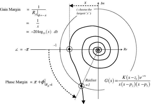
Figure 8.13 Gain margin and phase margin on a Nyquist plot.
8.6.5 Magnitude versus Phase-Angle Plot and the Nichols Chart
It is sometimes useful to use a ‘magnitude versus phase angle’ plot of the frequency response, as opposed to the Bode plot (Section 8.6.3) or Nyquist plot (Section 8.6.4). This is a Cartesian representation of the polar Nyquist plot, and it similarly loses information about frequency, unless frequencies are explicitly marked on the curve as in Figure 8.14. The system in Example 8.6 is plotted, and the corresponding closed-loop gain margin and phase margin now determined graphically.
![A graphical representation where open-loop amplitude ratio, RAO [db] is plotted on the y-axis on a scale of (-22)–(28) and openloop phase angle [degrees] on the x-axis on a scale of (-290)–(-71).](http://images-20200215.ebookreading.net/20/1/1/9783527341191/9783527341191__applied-process-control__9783527341191__images__c08__n8f014.gif)
Figure 8.14 Plot of open-loop amplitude ratio versus phase angle at a range of frequencies.
This type of plot is well known in another context, because a particular open-loop amplitude ratio and phase angle implies a particular closed-loop amplitude ratio and phase angle:
Consider an arbitrary point (RAO,ϕO) in this frequency response, where
Here the closed loop would map to
So,

Thus many different (RAO,ϕO) points in the plane could be used to compute the corresponding (RACL,ϕCL) values at those points, building two surfaces on which contours of constant RACL or ϕCL could be plotted. On the Nichols chart (Figure 8.15), both sets of these contours are shown simultaneously. The plot in Figure 8.14 is sometimes called a Nichols plot, and it can be superimposed on the Nichols chart as shown to give some direct insight into the closed-loop behaviour. One notes that the closed loop has a resonant peak at frequency ![]() 1 rad time−1 (i.e. where the plot is tangential to the constant RACL contours). A typical design criterion is to set this
1 rad time−1 (i.e. where the plot is tangential to the constant RACL contours). A typical design criterion is to set this
For the open-loop system of Equations 8.213 and 8.214, which is plotted in Figure 8.15, this requires a 2.5 db reduction in gain, that is KC must change such that the K = 5 in this expression becomes
![A graphical representation on the Nichols chart, where open-loop amplitude ratio, RAO [db] is plotted on the y-axis on a scale of (-22)–(28) and openloop phase angle [degrees] on the x-axis on a scale of (-290)–(-70).](http://images-20200215.ebookreading.net/20/1/1/9783527341191/9783527341191__applied-process-control__9783527341191__images__c08__n8f015.gif)
Figure 8.15 Plot of the open-loop system in Example 8.6 on the Nichols chart.
As seen, this will drop the entire open-loop curve by 2.5 db, giving the desired tangential contact with the 2 db closed-loop contour.
8.7 Control Quality Criteria
Most of the measures used to describe the performance of a controller refer to its setpoint step response as in Figure 8.16. Often this will be the basis for comparison of different settings or different controller algorithms. One appreciates that plant operators will not allow significant stepping in many installations, in which case more general measures such as ISE or IAE (see below) may have to be extracted from normal operating records over longer periods.
- Rise time time to reach setpoint value TR
- Overshoot expressed as a percentage

- Decay ratio ratio of successive amplitudes
 (related to closed-loop damping factor)
 - Settling time to a defined tolerance – for example 5% as shown: TS
- Offset not shown in this example, but obviously important in many proportional controllers. Here, one needs to obtain the mean initial output xSS1 (before the setpoint step) and the mean settling position xSS2. Then, the percentage offset is

Notice that this measure must be relative because the output is likely to start and end with an offset.
- Integrated error There are several different measures based on integrating the deviation from setpoint over some period of time following the setpoint step, but only two will be given here:
- ISE (integral of squared error) [also known as QPI (quadratic performance index)]
(8.229)

One might like to take t → ∞ as a good overall measure of performance, but since there will always be deviations in real situations, one is obliged to fix a finite T for comparison purposes. In the case of systems with offset, eliminate the prejudice of initial offset with
(8.230)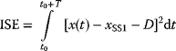
Obviously, if one is forced to compare indices based on different step sizes, the above expressions must be normalized with a factor of 1/D2. Bearing in mind the effects of nonlinearity, for comparison purposes a setpoint step should always be made between the same values and in the same direction.
- IAE (integral of absolute error)
(8.231)

Here, one can truly talk of ‘the area between the response curve and the setpoint’. The same points arise as under (a) with respect to T, offset and normalisation, except in the case of normalisation the factor will now be of 1/D.
- ISE (integral of squared error) [also known as QPI (quadratic performance index)]

Figure 8.16 Control quality measures based on a setpoint step response.
As mentioned, where actual steps are not allowed on the plant, real-time algorithms such as a ‘moving window’-based ISE could continuously monitor the setpoint deviation. Sophisticated methods exist, for example, that relate the setpoint deviation to simultaneous valve (actuator) movements, allowing the identification of valve hysteresis (see Section 2.6.1.5).
8.8 Robust Control
Since the 1980s a lot of work has been done on robust stability and robust performance. The problem being addressed here is that the design of a controller is based on a nominal model of a system – or at least on some fixed nominal behaviour of the equipment, sensors and actuators. So what happens when the operation at any time deviates from this behaviour? The aim is to build into the controller certain guarantees of the stability and performance, provided the deviations of the system from the nominal behaviour are within specified bounds. Interestingly, these techniques are developed in the more classical frequency domain. Since a good working knowledge of the field requires a significant mathematical background, this section will merely introduce some of the ideas.
In Figure 8.17, two means are proposed for incorporating an unknown model uncertainty, viz. additive [ΔP(s)], and multiplicative [Δ(s)], where it is understood that these deviation functions have a range of behaviour, for example as a result of their coefficients varying over some range. The corresponding open-loop transfer functions are
where
where
A single-frequency point on the Nyquist plot of ![]() is thus displaced in both cases, in magnitude and angle, by an uncertain function
is thus displaced in both cases, in magnitude and angle, by an uncertain function ![]() according to
according to
As an example, consider the particular case of a frequency ω1 at which the magnitude deviation factor and phase deviations are independent, and restricted to ranges 0.8 → 1.2 and −10° → + 10°, respectively (Figure 8.18). A transfer function having this behaviour would be of the form
where there is no uncertainty in ![]() but K could be from 20% smaller to 20% bigger, and the possible range of τ is such that
but K could be from 20% smaller to 20% bigger, and the possible range of τ is such that ![]() could be from 10° smaller to 10° bigger. Obviously if the uncertain terms lay in other places, such as the coefficients in
could be from 10° smaller to 10° bigger. Obviously if the uncertain terms lay in other places, such as the coefficients in ![]() , there would be interdependence of the magnitude and phase deviations, giving a more irregular shape. All these possible shapes representing the uncertainty range cannot be handled, so the practice is to simply approximate the uncertainty with a disc of radius ℓ(ω) centred at
, there would be interdependence of the magnitude and phase deviations, giving a more irregular shape. All these possible shapes representing the uncertainty range cannot be handled, so the practice is to simply approximate the uncertainty with a disc of radius ℓ(ω) centred at ![]() . Notice that ℓ(ω) is explicitly allowed to vary with ω because one expects a strong dependence of magnitude and phase angle, and thus the uncertainties thereof, on the frequency.
. Notice that ℓ(ω) is explicitly allowed to vary with ω because one expects a strong dependence of magnitude and phase angle, and thus the uncertainties thereof, on the frequency.
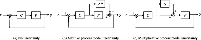
Figure 8.17 Representations of process model uncertainty.
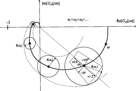
Figure 8.18 Uncertainty region of Nyquist plot point at frequencies ωi for independent magnitude and phase deviation ranges at these frequencies.
In Figure 8.18, it is thus seen that the allowance for uncertain deviations from the nominal ![]() defines a region on the complex plane containing all of the possible Nyquist plots of the uncertain system. One is immediately interested in whether this region includes or overlaps the point (−1 + j0). If it does not, the system is robustly stable. Of course, the same conditions apply as in Section 8.6.4: as ω decreases, the net positive encirclements of (−1 + j0) represent the number of positive real zeros minus positive real poles of
defines a region on the complex plane containing all of the possible Nyquist plots of the uncertain system. One is immediately interested in whether this region includes or overlaps the point (−1 + j0). If it does not, the system is robustly stable. Of course, the same conditions apply as in Section 8.6.4: as ω decreases, the net positive encirclements of (−1 + j0) represent the number of positive real zeros minus positive real poles of ![]() . First removing any negative rotationary contributions of open-loop unstable poles, if there is still an overlap of (−1 + j0) one can conclude that the closed loop lacks robust stability. Bearing in mind that nominal stability refers to the nominal transfer function
. First removing any negative rotationary contributions of open-loop unstable poles, if there is still an overlap of (−1 + j0) one can conclude that the closed loop lacks robust stability. Bearing in mind that nominal stability refers to the nominal transfer function ![]() , one notes that
, one notes that
- robust stability implies nominal stability;
- nominal stability does not necessarily imply robust stability;
- robust instability does not necessarily imply nominal instability; and
- nominal instability implies robust instability.
The proposed robust stability criterion requires that for all ω, the distance between the points ![]() and (−1 + j0) on the complex plane exceed ℓ(ω):
and (−1 + j0) on the complex plane exceed ℓ(ω):
The following discussion follows that of Damen and Weiland (2002). The uncertain control loops in Figure 8.17 can be represented as in Figure 8.19. This easily follows from
-
(8.242)

-
(8.243)

The terminology for the various transfer functions is sensitivity
(8.244)
control sensitivity
(8.245)
complementary sensitivity
(8.246)
Let M = −T. Then the Figure 8.19(b) can be represented as in Figure 8.20.

Figure 8.19 ‘Small gain’ representation of the impact of uncertainty in closed loop.

Figure 8.20 General small gain loop.
Small gain theorem: If Δ and M are stable, then the loop in Figure 8.20 is asymptotically stable if
In this condition, ![]() represents the infinity norm which for a SISO system H(s) is the maximum amplitude ratio in the frequency range
represents the infinity norm which for a SISO system H(s) is the maximum amplitude ratio in the frequency range
The equivalent expression for a MIMO system is
The ‘sup’ stands for supremum and effectively means the maximum of ![]() in the frequency range. The function
in the frequency range. The function ![]() denotes the largest singular value (always real) of the matrix of complex numbers
denotes the largest singular value (always real) of the matrix of complex numbers ![]() at any frequency ω.
at any frequency ω.
Notes
References
- Coughanowr, D.R. and Koppel, L.B. (1965) Process Systems Analysis and Control, McGraw-Hill.
- Damen, A. and Weiland, S. (2002) Robust Control, Measurement and Control Group, Department of Electrical Engineering, Eindhoven University of Technology, Draft version July 17, 2002.