
Chapter 8
Graphs
CHAPTER OUTLINE
8.1 INTRODUCTION
I want to meet Amitabh Bachchan. Do I know somebody who knows him? Or is there a path of connected people that can lead me to this great man? If yes, then how to represent the people and the path? The problem becomes challenging if the people involved are spread across various cities. For instance, my friend Mukesh from Delhi knows Surender at Indore who in turn knows Wadegoanker residing in Pune. Wadegoanker is a family friend of the great Sachin at Mumbai. The friendship of Sachin and Amitabh is known world over. There is an alternative given by Dr. Asok De. He says that his friend Basu from Kolkata is the first cousin of Aishwarya Rai, the daughter in law of Amitabh.
The various cities involved in this set of related people are connected by roads as shown Figure 8.1.
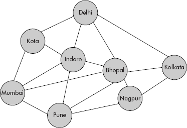
Fig. 8.1 Cities connected with roads
Now the problem is how to represent the data given in Figure 8.1. Arrays are linear by nature and every element in an array must have a unique successor and predecessor except the first and last elements. The arrangement shown in Figure 8.1 is not linear and, therefore, cannot be represented by an array. Though a tree is a non-linear data structure but it has a specific property that a node cannot have more than one parent. The arrangement of Figure 8.1 is not following any hierarchy and, therefore, there is no parent–child relationship.
A close look at the arrangement suggests that it is neither linear nor hierarchical but a network of roads connecting the participating cities. This type of structure is known as a graph. In fact, a graph is a collection of nodes and edges. Nodes are connected by edges. Each node contains data. For example, in Figure 8.1, the cities have been shown as nodes and the roads as edges between them. Delhi, Bhopal, Pune, Kolkata, etc. are nodes and the roads connecting them are edges. There are numerous examples where the graph can be used as a data structure. Some of the popular applications are as follows:
- Model of www: The model of world wide web (www) can be represented by a collection of graphs (directed) wherein nodes denote the documents, papers, articles, etc. and the edges represent the outgoing hyperlinks between them.
- Railway system: The cities and towns of a country are connected through railway lines. Similarly, road atlas can also be represented using graphs.
- Airlines: The cities are connected through airlines.
- Resource allocation graph: In order to detect and avoid deadlocks, the operating system maintains a resource allocation graph for processes that are active in the system.
- Electric circuits: The components are represented as nodes and the wires/connections as edges.
Graph: A graph has two sets: V and E, i.e., G = <V, E>, where V is the set of vertices or nodes and E is the set of edges or arcs. Each element of set E is a pair of elements taken from set V. Consider Figure 8.1 and identify the following:
V = {Delhi, Bhopal, Calcutta, Indore…․}
E = {(Delhi, Kota), (Bhopal, Nagpur), (Pune, Mumbai)…}
Before proceeding to discuss more on graphs, let us have a look at the basic terminology of graphs discussed in the subsequent section.
8.2 GRAPH TERMINOLOGY
In this book, the following terms related to graphs are used:
Directed graph: A directed graph is a graph G = <V, E> with the property that its edges have directions. An edge E: (vi, vj) means that there is an arrow whose head is pointing to vj and the tail to vi. A directed graph is shown in Figure 8.2(a). For example, (B, A), (A, D), (C, D), etc are directed edges. A directed graph is also called a diagraph.
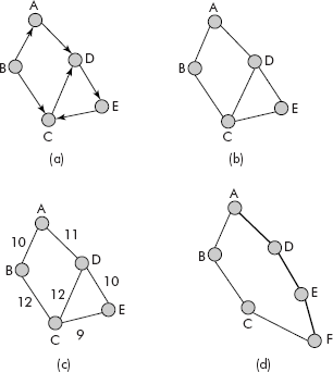
Fig. 8.2 Various kinds of graphs
Undirected graph: An undirected graph is a graph G = <V, E> with the property that its edges have no directions, i.e., the edges are two ways as shown in Figure 8.2(b). For example, (B, A), (A, B), etc. are two way edges. A graph always refers to an undirected graph.
Weighted graph: A weighted graph is a graph G = <V, E> with the property that its edges have a number or label associated with it. The number is called the weight of the edge. A weighted graph is shown in Figure 8.2(c). For example, (B, A) 10 may mean that the distance of B from A is 10m. A weighted graph can be an undirected graph or a directed graph.
Path: It is a sequence of nodes in which all the intermediate pair nodes between the first and the last nodes are joined by edges as shown in Figure 8.2(d). The path from A to F is shown with the help of dark edges. The path length is equal to the number of edges present in a path. The path length of A-D-E-F is 3 as it contains three edges.
However in the case of weighted graphs, the path length is computed as the sum of labels of the intermediate edges. For example, the path length of path A-D-C-E of Figure 8.2(c) is (11 + 12 + 9), i.e., 32.
It may be noted that if no node occurs more than once in a path then the path is called a sim-ple path. For example in Figure 8.2(b), A-B-C is a simple path. However, the path A-D-E-C-D is not a simple path.
Cycle: A path that starts and ends on the same node is called a cycle. For example, the path D- E-C-D in Figure 8.2(b) is a cycle.
Connected graph: If there exists a path be-tween every pair of distinct nodes, then the undirected graph is called a connected graph. For example, the graphs shown in Figures 8.3(b), (c) and (d) are connected graphs. How-ever, the graph shown in Figure 8.3(a) is not a connected graph.
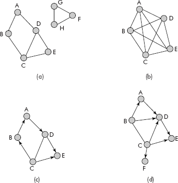
Fig. 8.3 More graphs
Adjacent node: A node Y is called adjacent to X if there exists an edge from X to Y. Y is called successor of X and X predecessor of Y. The set of nodes adjacent to X are called neighbours of X.
Complete graph: A complete graph is a graph G = <V, E> with the property that each node of the graph is adjacent to all other nodes of the graph, as shown in Figure 8.3(b).
Acyclic graph: A graph without a cycle is called an acyclic graph as shown in Figure 8.3(c). In fact, a tree is an excellent example of an acyclic graph.
Self loop: If the starting and ending nodes of an edge are same, then the edge is called a self loop, i.e., edge (E, E) is a self loop as shown in Figure 8.4(a).
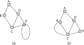
Fig. 8.4 Multigraphs
Parallel edges: If there are multiple edges between the same pair of nodes in a graph, then the edges are called parallel edges. For example, there are two parallel edges between nodes B and C of Figure 8.4(b).
Multigraphs: A graph containing self loop or parallel edges or both is called a multigraph. The graphs shown in Figure 8.4 are multigraphs.
Simple graph: A simple graph is a graph which is free from self loops and parallel edges.
Degree of a node or vertex: The number of edges connected to a node is called its degree. The maximum degree of a node in a graph is called the degree of the graph. For example, the degree of node A in Figure 8.3(a) is 2 and that of Delhi in Figure 8.1 is 4. The degree of graph in Figure 8.1 is 6.
However, in case of directed graphs, there are two degrees of a node—indegree and outdegree. The indgree is defined as the number of edges incident upon the node and outdegree as the number of edges radiating out of the node.
Consider Figure 8.3(d), the indegree and outdegree of C is 0 and 4, respectively. Similarly, the indegree and outdegree of D is 3 and 1, respectively.
Pendent node: A pendent node in a graph is a node whose indegree is 1 and outdegree is 0. The node F in Figure 8.3(d) is a pendent node. In fact, in a tree all leaf nodes are necessarily pendent nodes.
8.3 REPRESENTATION OF GRAPHS
A graph can be represented in many ways and the most popular methods are given below:
- Array-based representation
- Linked representation
- Set representation
These representations are discussed in detail in the sections that follow.
8.3.1 Array-based Representation of Graphs
A graph can be comfortably represented using an adjacency matrix implemented through a two-dimensional array. Adjacency matrix is discussed in detail below.
A graph of order N, i.e., having N nodes or vertices can be comfortably modelled as a square matrix N × N wherein the rows and the column numbers represent the vertices as shown in Figure 8.5.
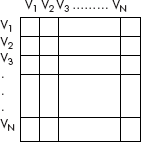
Fig. 8.5 A matrix representing a graph
A cell at the cross-section of vertices can have only Boolean values, 0 or 1. An entry (vi, vj) is 1 only when there exists an edge between vi and vj, otherwise a 0 indicates an absence of edge between the two.
The adjacency matrices for graphs of Figures 8.3(a–d) are given in Figure 8.6. From Figure 8.3(a), it may be observed that a row provides list of successors of a node and the column provides list of predecessors. The successors of B are A and C (see Figure 8.6(a)). An empty column under B suggests that there are no predecessors of B.
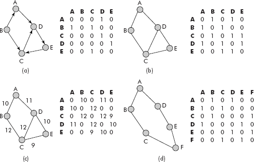
Fig. 8.6 The equivalent adjacency matrices for graphs
It may be noted that in the case of weighted graph (Figure 8.6 (d)), the edge weight has been stored instead of 1 to mark the presence of an edge. Some important properties of adjacency matrices are as follows:
Property 1: It may further be noted that the adjacency matrix is symmetric for an undirected graph.
This can be easily proved that an edge (vi, vj) of an undirected graph gets an entry into an adjacency matrix A at two locations: Aij and Aji. Thus in the matrix A for all i, j, Aij = Aji, which is the property of a symmetric matrix. Therefore, the following relation also holds good:
A = AT
where AT is the transpose of adjacency matrix A.
From Figure 8.6(a), it can be confirmed that in case of directed graphs, the adjacency matrix is not symmetric and therefore the following relation holds true.
A ≠ AT
However, for simple graphs, the diagonal elements are always 0.
Property 2: For a directed graph G with adjacency matrix A, the diagonal of matrix A × AT gives the out degrees of the corresponding vertices.
Consider the graph and its adjacency matrix A given in Figure 8.7.
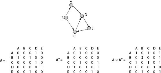
Fig. 8.7 The out degree of vertices denoted by diagonal elements of A × AT
It may be noted that the diagonal elements of AT × A are {1, 2, 1, 1, 1}, which are in fact the outdegrees of vertices A, B, C, D and E, respectively.
Similarly, for a directed graph G with adjacency matrix A, the diagonal of matrix AT × A gives the in degrees of the corresponding vertices. Consider the graph and its adjacency matrix A given in Figure 8.8.
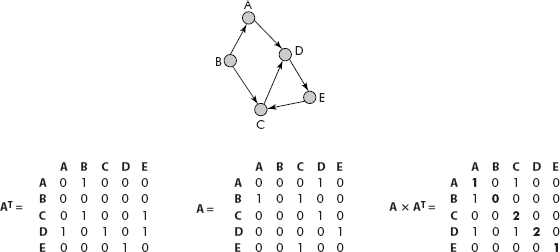
Fig. 8.8 The in degree of vertices denoted by diagonal elements of AT × A
It may be noted that the diagonal elements of AT × A are {1, 0, 2, 2, 1}, which are in fact the in degrees of vertices A, B, C, D and E, respectively.
Property 3: For a directed graph G with adjacency matrix A, the element Aij of matrix AK (kth power of A) gives the number of paths of length k from vertex vi to vj. This means that an element Aij of A2 will denote the number of paths of length 2 from vertex vi to vj. Consider Figure 8.9. A2 gives the path length of 2 from a vertex vi to vj. For example, there is one path of length 2 from C to A (i.e., C-B-A). Similarly, A3 gives the path length of 3 from a vertex vi to vj. For example, there is one path of length 3 from E to D (i.e., E-C-B-D).
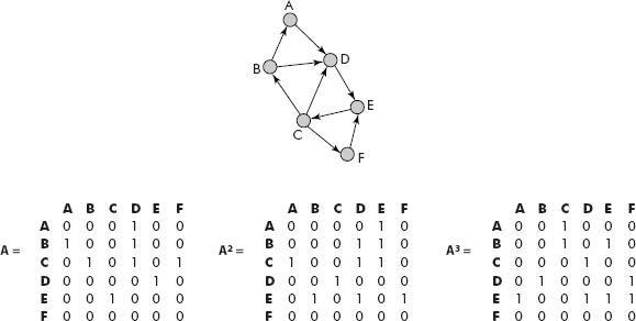
Fig. 8.9 Number of paths from a vertex to another vertex
The major drawback of adjacency matrix is that it requires N × N space whereas most of the entries in the matrix are 0, i.e., the matrix is sparse.
8.3.2 Linked Representation of a Graph
In order to save the space, an array of linked lists is used to represent the adjacent nodes and the data structure is called adjacency list. For example, the adjacency list for a directed graph is shown in Figure 8.10. Similarly, the adjacency list for an undirected graph is shown in Figure 8.11.
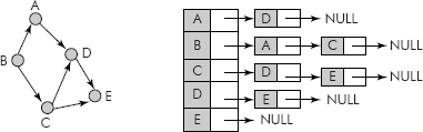
Fig. 8.10 Adjacency list for a directed graph
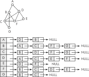
Fig. 8.11 Adjacency list for an undirected graph
The above representation involves a mix of array and linked lists, i.e., it is an array of linked lists. For pure linked representation, the array part can be replaced by another linked list of head nodes as shown in Figure 8.12. The head node contains three parts: data, pointer to adjacent node and a pointer to next head node as shown in Figure 8.13.
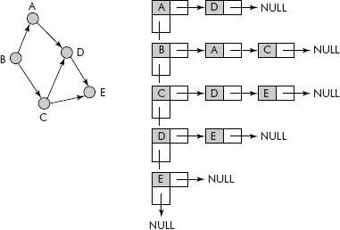
Fig. 8.12 The linked representation of an adjacency list of a directed graph
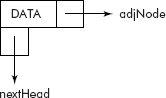
Fig. 8.13 The structure of a head node
Note: If in a graph G, there are N vertices and M edges, the adjacency matrix has space complexity O(N2) and that of adjacency list is O(M).
8.3.3 Set Representation of Graphs
This representation follows the definition of the graph itself in the sense that it maintains two sets: V- ‘Set of Vertices’ and E-’Set of Edges’. The set representation for various graphs is given in Figure 8.14.
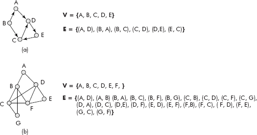
Fig. 8.14 The set representation of graphs
In case of weighted graphs, the weight is also included with the edge information making it a 3-tuple, i.e., (w, vi, vj) where w is the weight of edge between vertices vi and vj. The set representation for a weighted graph is given in Figure 8.15.
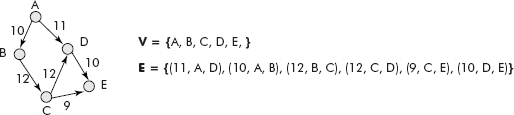
Fig. 8.15 The set representation of a weighted graph
This set representation is most efficient as far as storage is concerned but is not suitable for operations that can be defined on graphs. A discussion on operations on graphs is given in the section 8.4.
8.4 OPERATIONS OF GRAPHS
The following operations are defined on graphs:
- Insertion: There are two major components of a graph—vertex and edge. Therefore, a node or an edge or both can be inserted into an existing graph.
- Deletion: Similarly, a node or an edge or both can be deleted from an existing graph.
- Traversal: A graph may be traversed for many purposes—to search a path, to search a goal, to establish a shortest path between two given nodes, etc.
8.4.1 Insertion Operation
The insertion of a vertex and its associated edge with other vertices in an adjacency matrix involves the following operations:
- Add a row for the new vertex.
- Add a column for the new vertex.
- Make appropriate entries into the rows and columns of the adjacency matrix for the new edges.
Consider the graph given in Figure 8.16.
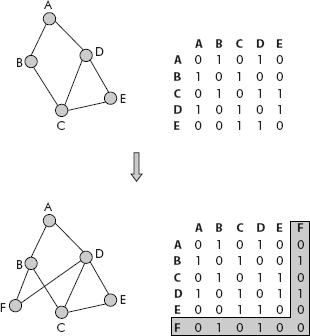
Fig. 8.16 Insertion of a vertex into an undirected graph
It may be noted that a vertex called F has been added to the graph. It has two edges (F, B) and (F, D). The adjacency matrix has been accordingly modified to have a new row and a new column for the incoming vertex. Appropriate entries for the edges have been made in the adjacency matrix, i.e., the cells (F, B), (F, D), (B, F) and (D, F) have been set equal to 1.
An algorithm for insertion of a vertex is given below:
  /* This algorithm uses a two-dimensional matrix adjMat[][] to store the adjacency matrix.
  A new vertex called verTex is added to the matrix by adding an additional empty
  row and an additional empty column. */
  Algorithm addVertex ()
  {
   lastRow = lastRow + 1;
   lastCol = lastCol + 1;
   adjMat[lastRow][0] = verTex;
   adjMat[0][lastCol] = verTex;
   Set all elements of last row = ’0’;
   Set all elements of last Col = ’0’;
  }
An algorithm for insertion of an edge into an undirected graph is given below:
  /* This algorithm uses a two-dimensional matrix adjMat[][] to store the adjacency
  matrix. A new edge (v1, v2) is added to the matrix by adding its entry
  (i.e., ’1’) in the row and column corresponding to v1 and v2, respectively. */

  Algorithm addEdge()
  {
    Find row corresponding to v1, i.e., rowV1;
    Find col corresponding to v2, i.e., colV2;
    adjMat[rowV1][ColV2] = ’1’;         /* make symmetric entries */
    adjMat[colV2][rowV1] = ’1’;
  }
Example 1: Write a program that implements an adjacency matrix wherein it adds a vertex and its associated edges. The final adjacency matrix is displayed.
Solution: Two functions called addVertex() and addEdge() would be used for insertion of a new vertex and its associated edges, respectively. Another function called dispAdMat() would display the adjacency matrix.
The required program is given below:
  /* This program implements an adjacency matrix */
  #include <stdio.h>
  #include <conio.h>
  void addVertex (char adjMat[7][7], int numV, char verTex);
  void addEdge (char adjMat[7][7], char v1, char v2, int numV);
  void dispAdMat(char adjMat[7][7], int numV);
  void main()
  {                /* Adjacency matrix of Figure 8.17 */
    char adjMat[7][7] = { ’-’,  ’A’,’B’,’C’,’D’,’E’,’ ’,
    ’A’, ’0’, ’1’, ’0’, ’1’, ’0’,’ ’,
    ’B’, ’1’, ’0’, ’1’,’0’, ’0’,’ ’,
    ’C’, ’0’, ’1’, ’0’,’1’, ’1’,’ ’,
    ’D’, ’1’, ’0’, ’1’,’0’, ’1’,’ ’,
    ’E’, ’0’, ’0’, ’1’,’1’, ’0’,’ ’,
    ’ ’, ’ ’, ’ ’, ’ ’, ’ ’, ’ ’, ’ ’};
    int numVertex = 5;
    char newVertex, v1,v2;
    char choice;
    dispAdMat (adjMat, numVertex);

    printf (“
 Enter the vertex to be added”);
    fflush (stdin);
    newVertex = getchar();
    numVertex++; addVertex
    (adjMat, numVertex, newVertex);
    do
    {
      fflush(stdin);
      printf (“
 Enter Edge: v1 - v2”);
      scanf (“%c %c”, &v1, &v2);
      addEdge (adjMat, v1,v2,numVertex);
      dispAdMat (adjMat, numVertex);
      fflush (stdin);
      printf (“
 do you want to add another edge Y/N”);
      choice = getchar();
    }
    while ((choice != ’N’) && (choice != ’n’));
  }
  void addVertex (char adjMat[7][7], int numV, char verTex)
  { int i;
    adjMat[numV][0] = verTex;
    adjMat[0][numV] = verTex;
    for (i = 1; i<= numV; i++)
    {
      adjMat[numV][i] = ’0’;
      adjMat[i][numV] = ’0’;
    }
  }
  void addEdge (char adjMat[7][7], char v1, char v2, int numV)
  { int i, j, k;
    i = 0;
    for (j = 1; j <= numV; j++)
    {
      if (adjMat[i][j] == v1)
      {
        for (k = 0; k <= numV; k++)
        {
          if (adjMat [k][0] == v2)
          {
            adjMat[k][j] = ’1’;
            adjMat[j][k] = ’1’; break; /* making symmetric entries */
          }
        }
      }
    }
  }

  void dispAdMat(char adjMat[7][7], int numV)
  {
    int i,j;
    printf (“
The adj Mat is--
”);
    for (i=0; i<= numV; i++)
    {
      for (j=0; j<=numV; j++)
      {
        printf (“%c ”, adjMat[i][j]);
      }
      printf (“
”);
    }
    printf (“

 Enter any key to continue”);
    getch();
  }
The above program has been tested for data given in Figure 8.16. The screenshots of the result are given in Figure 8.17.
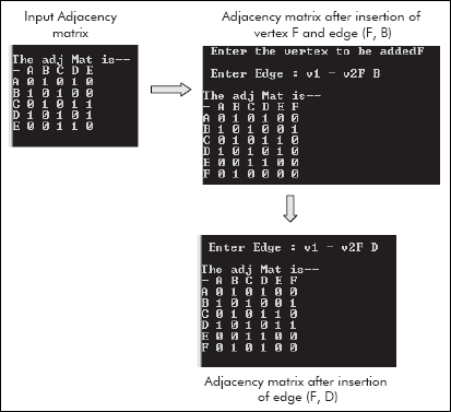
Fig. 8.17 The adjacency matrix before and after insertion of vertex F
Note: In case of a directed graph, only one entry of the directed edge in the adjacency matrix needs to be made. An algorithm for insertion of a vertex in a directed graph is given below:
  /* This algorithm uses a two-dimensional matrix adjMat[][] to store the
  adjacency matrix. A new vertex called verTex is added to the matrix by
  adding an additional empty row and an additional empty column. */
  Algorithm addVertex ()
  {
   lastRow = lastRow + 1;
   lastCol = lastCol + 1;
   adjMat[lastRow][0] = verTex;
   adjMat[0][lastCol] = verTex;
   Set all elements of last row = ’0’;
   Set all elements of last Col = ’0’;
  }
An algorithm for insertion of an edge into a directed graph is given below:
  /* This algorithm uses a two-dimensional matrix adjMat[][] to store the
  adjacency matrix. A new edge (v1, v2) is added to the matrix by adding its
  entry (i.e., ’1’) in the row corresponding to v1. */
  Algorithm addEdge ()
  {
    Find row corresponding to v1, i.e., rowV1;
    Find col corresponding to v2, i.e., colV2;
    adjMat[rowV1][ColV2] = ’1’;
  }
Accordingly, the function addEdge() needs to modified so that it makes the adjacency matrix assymmetric. The modified function is given below:
  /* The modified function for addition of edges in directed graphs */
  void addEdge (char adjMat[7][7], char v1, char v2, int numV)
  { int i,j, k;
    j=0;
    for (i=1; i<=numV; i++)
    {
      if (adjMat[i][j] == v1)
      {
        for (k=1; k<= numV; k++)
        {
          if (adjMat [0][k] ==v2)
          {
            adjMat[i][k] = ’1’; break;
          }
        }
      }
    }
  }
8.4.2 Deletion Operation
The deletion of a vertex and its associated edges from an adjacency matrix, for directed and undirected graph, involves the following operations:
- Deleting the row corresponding to the vertex.
- Deleting the col corresponding to the vertex.
The algorithm is straight forward and given below:
  Algorithm  delVertex (verTex)
  {
    find the row corresponding to verTex and set all its elements = ’0’;
    find the col corresponding to verTex and set all its elements = ’0’;
  }
The deletion of an edge from a graph requires different treatment for undirected and directed graphs. Both the cases of deletion of edges are given below:
An algorithm for deletion of an edge from an undirected graph is given below:
  /* This algorithm uses a two-dimensional matrix adjMat[][] to store the
  adjacency matrix. A new edge (v1, v2) is deleted from the matrix by
  deleting its entry (i.e., ’0’) from the row and column corresponding to v1
  and v2, respectively. */
  Algorithm delEdge ()               /* undirected graph */
  {
    Find row corresponding to v1, i.e., rowV1;
    Find col corresponding to v2, i.e., colV2;
    adjMat[rowV1][ColV2] = ’0’;   /* make symmetric entries */
    adjMat[colV2][rowV1] = ’0’;
  }
An algorithm for deletion of an edge from a directed graph is given below:
  /* The algorithm uses a two-dimensional matrix adjMat[][] to store the
  adjacency matrix. An edge (v1, v2) is deleted from the matrix by deleting
  its entry (i.e., ’0’) from the row corresponding to v1 */
  Algorithm delEdge()               /* directed graph */
  {
    Find row corresponding to v1, i.e., rowV1;
    Find col corresponding to v2, i.e., colV2;
    adjMat[rowV1][ColV2] = ’0’;
  }
Example 2: Write a program that deletes a vertex and its associated edges from an adjacency matrix. The final adjacency matrix is displayed.
Solution: A function called delVertex() would be used for deletion of a vertex and its associated edges from an adjacency matrix. Another function called dispAdMat() would display the adjacency matrix.
The required program is given below:
  /* This program deletes a vertex from an adjacency list */

  #include <stdio.h>
  #include <conio.h>

  void delVertex (char adjMat[7][7], int numV, char verTex);
  void dispAdMat (char adjMat[7][7], int numV);

  void main()
  {
    char adjMat[7][7] = { ’-’, ’A’,’B’,’C’,’D’,’E’,’ ’,
         ’A’, ’0’, ’1’, ’0’, ’1’, ’0’,’ ’,
         ’B’, ’1’, ’0’, ’1’,’0’, ’0’,’ ’,
         ’C’, ’0’, ’1’, ’0’,’1’, ’1’,’ ’,
         ’D’, ’1’, ’0’, ’1’,’0’, ’1’,’ ’,
         ’E’, ’0’, ’0’, ’1’,’1’, ’0’,’ ’,
         ’ ’, ’ ’, ’ ’, ’ ’, ’ ’, ’ ’, ’ ’};
    int numVertex = 5;
    char Vertex;
    dispAdMat (adjMat, numVertex);
    printf (“
 Enter the vertex to be deleted”);
    fflush (stdin);
    Vertex=getchar();
    delVertex (adjMat, numVertex, Vertex);
    dispAdMat (adjMat, numVertex);
  }
  void delVertex (char adjMat[7][7], int numV, char verTex)
  { int i, j, k;
  j = 0;
  for (i = 1; i <= numV; i++)
  {
      if (adjMat[i][j] == verTex)
      {
        adjMat[i][0] =’-’;
        for (k = 1; k <= numV; k++)
        {
          adjMat[i][k] = ’0’;
        }
      }
  }
  i = 0;
  for (j = 1; j <= numV; j++)
  {
      if (adjMat[i][j] == verTex)
      {
        adjMat[0][j] = ’-’;
        for (k = 1; k <= numV; k++)

        {
          adjMat[k][j] = ’0’;
        }
      }
  }
  }
  void dispAdMat(char adjMat[7][7], int numV)
  {
    int i, j;
    printf (“
The adj Mat is--
”);
    for (i = 0; i <= numV; i++)
    {
      for (j = 0; j <= numV; j++)
      {
        printf (“%c ”, adjMat[i][j]);
      }
      printf (“
”);
    }
    printf (“

 Enter any key to continue”);
    getch();
  }
The screenshots of the output of the program are shown in Figure 8.18.
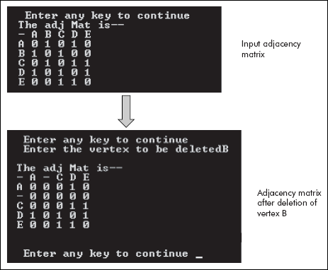
Fig. 8.18 The adjacency matrix before and after deletion of vertex B
Example 3: Write a program that deletes an edge from an adjacency matrix of an undirected graph. The final adjacency matrix is displayed.
Solution: A function called delEdge() would be used for deletion of an edge from an adjacency ma-trix. Another function called dispAdMat() would display the adjacency matrix.
The required program is given below:
  /* This program deletes an edge of an undirected graph from an adjacency matrix */
  #include <stdio.h>
  #include <conio.h>
  void delEdge (char adjMat[7][7], char v1, char v2, int numV);
  void dispAdMat(char adjMat[7][7], int numV);
  void main()
  {
    char adjMat[7][7] = { ’-’, ’A’,’B’,’C’,’D’,’E’,’ ’,
         ’A’, ’0’, ’1’, ’0’, ’1’, ’0’,’ ’,
         ’B’, ’1’, ’0’, ’1’,’0’, ’0’,’ ’,
         ’C’, ’0’, ’1’, ’0’,’1’, ’1’,’ ’,
         ’D’, ’1’, ’0’, ’1’,’0’, ’1’,’ ’,
         ’E’, ’0’, ’0’, ’1’,’1’, ’0’,’ ’,
         ’ ’, ’ ’, ’ ’, ’ ’, ’ ’, ’ ’, ’ ’};
    int numVertex = 5;
    char v1, v2;
    dispAdMat (adjMat, numVertex);
    printf (“
 Enter the edge to be deleted”);
    fflush (stdin);
    printf (“
 Enter Edge : v1 - v2”);
    scanf (“%c %c”, &v1, &v2);
    delEdge (adjMat, v1,v2,numVertex);
    dispAdMat (adjMat, numVertex);
  }
  void delEdge (char adjMat[7][7], char v1, char v2, int numV)
  { int i, j, k;
  i = 0;
  for (j = 1; j <= numV; j++)
  {
      if (adjMat[i][j] == v1)
      {
        for (k = 0; k <= numV; k++)
        {
          if (adjMat [k][0] == v2)
          {
            adjMat[k][j] = ’0’;
            adjMat[j][k] = ’0’; break; /* making symmetric entries */

          }
        }
      }
  }
  }

  void dispAdMat(char adjMat[7][7], int numV)
  {
    int i,j;
    printf (“
The adj Mat is--
”);
    for (i=0; i<= numV; i++)
    {
      for (j=0; j<=numV; j++)
      {
        printf (“%c ”, adjMat[i][j]);
      }
      printf (“
”);
    }
    printf (“

 Enter any key to continue”);
    getch();
  }
The screenshots of the output of the program are given in Figure 8.19.
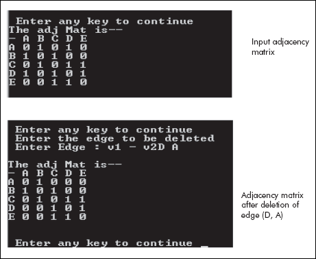
Fig. 8.19 The adjacency matrix before and after deletion of edge (D,A)
The function delEdge () needs to modified for directed graphs so that it does not make the adjacency matrix as symmetric. The modified function is given below:
  /* The modified function for deletion of edges of directed graphs */
  void delEdge (char adjMat[7][7], char v1, char v2, int numV)
  { int i, j, k;
  j = 0;
  for (i = 1; i <= numV; i++)
  {
      if (adjMat[i][j] == v1)
      {
        for (k = 1; k <= numV; k++)
        {
          if (adjMat [i][k] == v2)
          {
            adjMat[i][k] = ’0’;break;
          }
        }
      }
  }
  }
8.4.3 Traversal of a Graph
Travelling a graph means that one visits the vertices of a graph at least once. The purpose of the travel depends upon the information stored in the graph. For example on www, one may be interested to search a particular document on the Internet while on a resource allocation graph the operating system may search for deadlocked processes.
In fact, search has been used as an instrument to find solutions. The epic ‘Ramayana’ uses the search of goddess ‘Sita’ to find and settle the problem of ‘Demons’ of that yuga including ‘Ravana’. Nowadays, the search of graphs and trees is very widely used in artificial intelligence.
A graph can be traversed in many ways but there are two popular methods which are very widely used for searching graphs; they are: Depth First Search (DFS) and Breadth First Search (BFS). A detailed discussion on both is given in the subsequent sections.
8.4.3.1 Depth First Search (DFS)
In this method, the travel starts from a vertex then carries on to its successors, i.e., follows its outgoing edges. Within successors, it travels their successor and so on. Thus, this travel is same as inorder travel of a tree and, therefore, the search goes deeper into the search space till no successor is found. Once the search space of a vertex is exhausted, the travel for next vertex starts. This carries on till all the vertices have been visited. The only problem is that the travel may end up in a cycle. For example, in a graph, there is a possibility that the successor of a successor may be the vertex itself and the situation may end up in an endless travel, i.e., a cycle.
In order to avoid cycles, we may maintain two queues: notVisited and Visited. The vertices that have already been visited would be placed on Visited. When the successors of a vertex are generated, they are placed on notVisited only when they are not already present on both Visited and notVisited queues thereby reducing the possibility of a cycle.
Consider the graph shown in Figure 8.20. The trace of DFS travel of the given graph is given in Figures 8.20 and 8.21, through entries into the two queues Visited and notVisited.
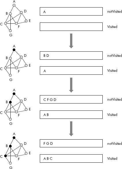
Fig. 8.20 The trace of DFS travel of a graph
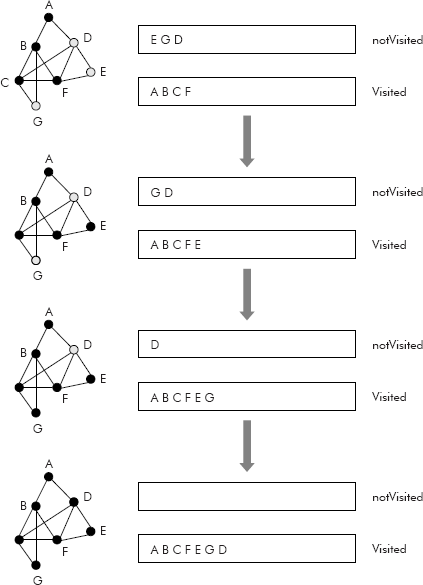
Fig. 8.21 The trace of DFS travel of a graph
The algorithm for DFS travel is given below:
Algorithm DFS (firstVertex)
{
  add firstVertex on notVisited;
  place NULL on Visited;          /* initially Visited is empty */
  while (notVisited != NULL)
  {
    remove vertex from notVisited;
    generate successors of vertex ;
    for each successor of vertex do
    {
      if (successor is not present on Visited AND successor is not present
      on notVisited) Then add vertex on front of notVisited;
    }

  if (vertex is not present on Visited) Then add vertex on Visited;
  }
}
The final visited queue contains the nodes visited during DFS travel, i.e., A B C F E G D.
Example 4: Write a program that travels a given graph using DFS strategy.
Solution: We would use the following functions:
(1) void addNotVisited (char Q[], int *first, char vertex); :
This function adds a vertex on notVisited queue in front of the queue.
(2) void addVisited (char Q[], int *last, char vertex);
This function adds a vertex on Visited queue.
(3) char removeNode (char Q[], int *first);
This function removes a vertex from notVisited queue.
(4) int findPos (char adjMat[8][8], char vertex);
This function finds the position of a vertex in adjacency matrix, i.e., adjMat.
(5) void dispAdMat(char adjMat[8][8], int numV);
This function displays the contents of adjacency matrix, i.e., adjMat.
(6) int ifPresent (char Q[], int last, char vertex);
This function checks whether a vertex is present on a queue or not.
(7) void dispVisited (char Q[], int last);
This function displays the contents of Visited queue.
We would use the adjacency matrix of graph shown in Figures 8.20 and 8.21. The required program is given below:
/* This program travels a graph using DFS strategy */

#include <stdio.h>
#include <conio.h>

void addNotVisited (char Q[], int *first, char vertex);
void addVisited (char Q[], int *last, char vertex);
char removeNode (char Q[], int *first);
int findPos (char adjMat[8][8], char vertex);
void dispAdMat(char adjMat[8][8], int numV);
int ifPresent (char Q[], int last, char vertex);
void dispVisited (char Q[], int last);
void main()
{ int i,j, first, last, pos;
char adjMat[8][8] = { ’-’, ’A’, ’B’, ’C’, ’D’, ’E’,’F’,’G’,
       ’A’, ’0’, ’1’, ’0’, ’1’, ’0’,’0’,’0’,
       ’B’, ’1’, ’0’, ’1’, ’0’, ’0’,’1’,’1’,
       ’C’, ’0’, ’1’, ’0’, ’1’, ’0’,’1’,’1’ ,
       ’D’, ’1’, ’0’, ’1’, ’0’, ’1’,’1’,’0’ ,
       ’E’, ’0’, ’0’, ’0’, ’1’, ’0’,’1’,’0’ ,
       ’F’, ’0’, ’1’, ’1’, ’1’, ’1’,’0’,’0’,
       ’G’, ’0’, ’1’, ’1’, ’0’, ’0’,’0’,’0’};
int numVertex = 7;
char visited [7], notVisited [7];
char vertex, v1,v2;
clrscr();
dispAdMat (adjMat, numVertex);
first = 7;
last =−1;
addNotVisited (notVisited , &first, adjMat[1][0]);
while (first < 7)
{
   vertex = removeNode (notVisited, &first);
   if (! ifPresent(visited, last, vertex))
       addVisited( visited,&last, vertex);

   pos =findPos (adjMat, vertex);
   for (i = 7; i>= 1; i−−)
   {
     if (adjMat[pos][i] == ’1’)
     {
       if (! ifPresent(notVisited, 7, adjMat[0][i]) &&
           (! ifPresent(visited, 7, adjMat[0][i]) ))
           addNotVisited( notVisited,&first, adjMat[0][i]);
     }
   }
}
printf (“
 Final visited nodes...”);
dispVisited (visited, last);
}

void dispAdMat(char adjMat[8][8], int numV)
{
  int i,j;
  printf (“
The adj Mat is--
”);
  for (i=0; i<= numV; i++)
  {
    for (j=0; j<=numV; j++)
    {
      printf (“%c ”, adjMat[i][j]);
    }
    printf (“
”);
  }
  printf (“

 Enter any key to continue ”);
  getch();
}

/* This function checks whether a vertex is present on a Q or not */
int ifPresent (char Q[], int last, char vertex)
{

  int i, result=0;
  for (i=0; i<= last; i++)
  {
    if (Q[i] == vertex)
    { result= 1;
    break;}
  }
  return result;
}
void addVisited (char Q[], int *last, char vertex)
{
  *last = *last + 1;
  Q[*last] = vertex;
}
void addNotVisited (char Q[], int *first, char vertex)
{
  *first = *first − 1;
  Q[*first] = vertex;
}
void dispVisited (char Q[], int last)
{
  int i;
  printf (“
 The visited nodes are ...”);
  for (i =0; i <= last; i++)
    printf (“ %c ”, Q[i]);
}

char removeNode (char Q[], int *first)
{
  char ch;
  ch = Q[*first];
  Q[*first] = ’#’;
  *first = *first + 1;
  return ch;
}
int findPos (char adjMat[8][8], char vertex)
{
  int i;
  for (i = 0; i <= 7; i++)
  {
    if (adjMat[i][0]==vertex)
        return i;
  }
  return 0;
}
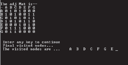
The output of the program is shown in Figure 8.22. The final list of visited nodes matches with the results obtained in Figures 8.20 and 8.21, i.e., the visited nodes are A B C F G D E.
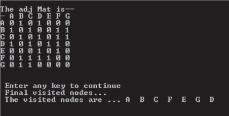
Fig. 8.22 The output of DFS travel
8.4.3.2 Breadth First Search (BFS)
In this method, the travel starts from a vertex then carries on to its adjacent vertices, i.e., follows the next vertex on the same level. Within a level, it travels all its siblings and then moves to the next level. Once the search space of a level is exhausted, the travel for the next level starts. This carries on till all the vertices have been visited. The only problem is that the travel may end up in a cycle. For example, in a graph, there is a possibility that the adjacent of an adjacent may be the vertex itself and the situation may end up in an endless travel, i.e., a cycle.
In order to avoid cycles, we may maintain two queues—notVisited and Visited. The vertices that have already been visited would be placed on Visited. When the successor of a vertex are generated, they are placed on notVisited only when they are not already present on both Visited and notVisited queues, thereby reducing the possibility of a cycle.
Consider the graph given in Figure 8.23. The trace of BFS travel of the given graph is given in Figures 8.23 and 8.24, through entries into the two queues—Visited and notVisited.
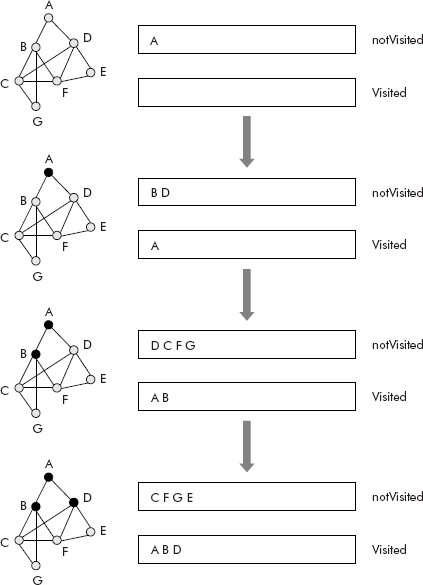
Fig. 8.23 The trace of BFS travel of a graph
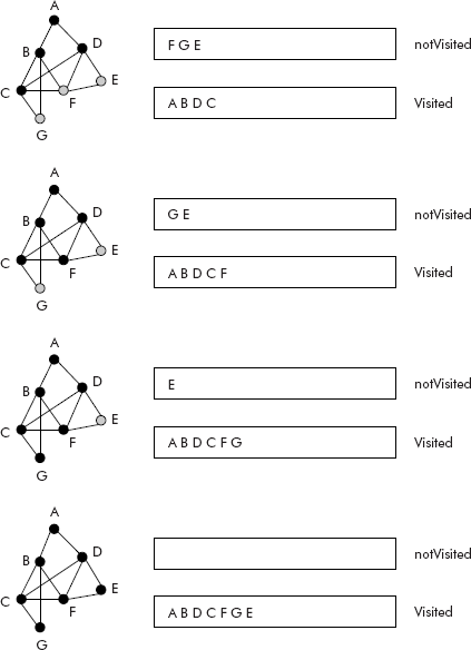
Fig. 8.24 The trace of BFS travel of a graph
The Visited queue contains the nodes visited during BFS travel, i.e., A B D C F G E.
The algorithm for BFS travel is given below:
  Algorithm BFS (firstVertex)
 {
  add firstVertex on notVisited;
  place NULL on Visited; /* initially Visited is empty */
  while (notVisited ! = NULL)
  {
    remove vertex from notVisited;
    generate adjacents of vertex;
    for each adjacent of vertex do
    {
      if (adjacent is not present on Visited AND adjacent is not present on notVisited) Then add adjacent at Rear on notVisited;
    }
    if (vertex is not present on Visited) Then add vertex on Visited;
  }
}
Example 5: Write a program that travels a given graph using breadth first search strategy.
Solution: We would use the following functions:
(1) void addNotVisited (char Q[], int *first, char vertex); :
This function adds a vertex on notVisited queue at Rear of the queue.
(2) void addVisited (char Q[], int *last, char vertex);
(3) char removeNode (char Q[], int *first);
(4) int findPos (char adjMat[8][8], char vertex);
(5) void dispAdMat(char adjMat[8][8], int numV);
(6) int ifPresent (char Q[], int last, char vertex);
(7) void dispVisited (char Q[], int last);
The purpose of the above functions has been explained in Example 4. The function addNotVisited() has been slightly modified.
The adjacency matrix of graph shown in Figures 8.20 and 8.21 is used. The program of Example 4 has been suitably modified which is given below:
/* This program travels a graph using BFS strategy */

#include <stdio.h>
#include <conio.h>

void addNotVisited (char Q[], int *first, char vertex);
void addVisited (char Q[], int *last, char vertex);
char removeNode (char Q[], int *first);
int findPos (char adjMat[8][8], char vertex);
void dispAdMat(char adjMat[8][8], int numV);
int ifPresent (char Q[], int last, char vertex);
void dispVisited (char Q[], int last);
void main()
{ int i,j, first, last, pos, Rear;
  char adjMat[8][8] = { ’-’, ’A’, ’B’, ’C’, ’D’, ’E’,’F’,’G’,
       ’A’, ’0’, ’1’, ’0’, ’1’, ’0’,’0’,’0’,
       ’B’, ’1’, ’0’, ’1’, ’0’, ’0’,’1’,’1’,
       ’C’, ’0’, ’1’, ’0’, ’1’, ’0’,’1’,’1’ ,
       ’D’, ’1’, ’0’, ’1’, ’0’, ’1’,’1’,’0’ ,
       ’E’, ’0’, ’0’, ’0’, ’1’, ’0’,’1’,’0’ ,
       ’F’, ’0’, ’1’, ’1’, ’1’, ’1’,’0’,’0’,
       ’G’, ’0’, ’1’, ’1’, ’0’, ’0’,’0’,’0’};
  int numVertex = 7;
  char visited [7], notVisited [7];

  char vertex, v1, v2;
  clrscr();
  dispAdMat (adjMat, numVertex);
  first = −1;
  Rear = −1;
  last =−1;
  addNotVisited (notVisited , &Rear, adjMat[1][0]);
  while (first <= Rear )
  {
    vertex = removeNode (notVisited, &first);
    if (! ifPresent(visited, last, vertex))
    addVisited( visited,&last, vertex);

    pos =findPos (adjMat, vertex);
    for (i = 1; i<= 7; i++)
    {
      if (adjMat[pos][i] == ’1’)
      {
        if (! ifPresent(notVisited, 7, adjMat[0][i]) &&
           (! ifPresent(visited, 7, adjMat[0][i]) ))

        {
          addNotVisited( notVisited,&Rear, adjMat[0][i]);
        }
      }
    }
  }
printf (“
 Final visited nodes...”);
dispVisited (visited, last);
}

void dispAdMat(char adjMat[8][8], int numV)
{
  int i,j;
  printf (“
The adj Mat is--
”);
  for (i=0; i<= numV; i++)
  {
    for (j=0; j<=numV; j++)
    {
      printf (“%c ”, adjMat[i][j]);
    }
    printf (“
”);
  }
  printf (“

 Enter any key to continue ”);
  getch();
}

/* This function checks whether a vertex is present on a Q or not */
int ifPresent (char Q[], int last, char vertex)
{
  int i, result = 0;
  for (i = 0; i <= last; i++)
  {
    if (Q[i] == vertex)
    { result = 1;
      break;}
  }
  return result;
}

void addVisited (char Q[], int *last, char vertex)
{
  *last = *last + 1;
  Q[*last] = vertex;
}
void addNotVisited (char Q[], int *Rear, char vertex)
{
  *Rear = *Rear + 1;
  Q[*Rear] = vertex;
}
void dispVisited (char Q[], int last)
{
  int i;
  printf (“
 The visited nodes are ...”);
  for (i =0; i <= last; i++)
  {
    printf (“ %c ”, Q[i]);
  }
}
char removeNode (char Q[], int *first)
{
  char ch;
  ch = Q[*first];
  Q[*first] = ’#’;
  *first = *first + 1;
  return ch;
}
int findPos (char adjMat[8][8], char vertex)
{
  int i;
  for (i = 0; i <= 7; i++)
  {
    if (adjMat[i][0]==vertex)
        return i;
  }
  return 0;
}
The output of the program is shown in Figure 8.25. The final list of visited nodes matches with the results obtained in Figures 8.23 and 8.24, i.e., the visited nodes are A B D C F G E.
Note: Implementation of operations on graphs using adjacency matrix is simple as compared to adjacency list. In fact, adjacency list would require the extra overhead of maintaining pointers. Moreover, the linked lists connected to vertices are independent and it would be difficult to establish cross-relationship between the vertices contained on different lists, which is otherwise possible by following a column in adjacency matrix.
8.4.4 Spanning Trees
A connected undirected graph has the following two properties:
- There exists a path from every node to every other node.
- The edges have no associated directions.
For example, the graph shown in Figure 8.26 is a connected undirected graph.
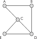
Fig. 8.26 A connected undirected graph
We know that a tree is a special graph which does not contain a cycle. Thus, we can remove some edges from the graph of Figure 8.26 such that it is still connected but has no cycles. The various sub-graphs or trees so obtained are shown in Figure 8.27.
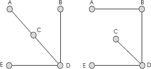
Fig. 8.27 The acyclic sub-graphs or trees
Each tree shown in Figure 8.27 is called a spanning tree of the graph given in Figure 8.26. Precisely, we can define a spanning tree of a graph G as a connected sub-graph, containing all vertices of G, with no cycles. It may be noted that there will be exactly n-1 edges in a spanning tree of a graph G having n vertices. Since a spanning tree has very less number of edges, it is also called as a sparse graph.
A graph can be traveled in two ways: Breadth First Search (BFS) and Depth First Search (DFS). In these travels, the cycles are avoided. Therefore the travels result in two trees: BFS-spanning tree and DFS-spanning trees. The DFS and BFS spanning trees corresponding to graph of Figure 8.26 are given in Figure 8.28
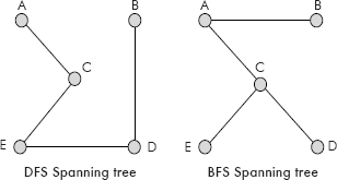
Fig. 8.28 DFS and BFS spanning trees
8.4.4.1 Minimum Cost Spanning Trees
From previous section, we know that multiple spanning trees can be drawn from a connected undirected graph. If it is weighted graph then the cost of each spanning tree can be computed by adding the weights of all the edges of the spanning tree. If the weights of the edges are unique then there will be one spanning tree whose cost is minimum of all. The spanning tree with minimum cost is called as minimum spanning tree or Minimum-cost Spanning Tree (MST).
Having introduced the spanning trees, lets us now see where they can be applied. An excellent situation that comes to mind is a housing colony wherein the welfare association is interested to lay down the electric cables, telephone lines and water pipelines. In order to optimize, it would be advisable to connect all the houses with minimum number of connecting lines. A critical look at the situation indicates that a spanning tree would be an ideal tool to model the connectivity layout. In case the houses are not symmetrical or are not uniformly distanced then an MST can be used to model the connectivity layout. Computer network cabling layout is another example where an MST can be usefully applied.
There are many algorithms available for finding an MST. However, following two algorithms are very popular.
- Kruskal’s algorithm
- Prim’s algorithm
A detailed discussion on these algorithms is given below:
Kruskal’s algorithm: In this algorithm, the edges of graph of n nodes are placed in a list in ascending order of their weights. An empty spanning tree T is taken. The smallest edge is removed from the list and added to the tree only if it does not create a cycle. The process is repeated till the number edges is less than or equal to n-1 or the list of edges becomes empty. In case the list becomes empty, then it is inferred that no spanning tree is possible.
Consider the graph given in Figure 8.29
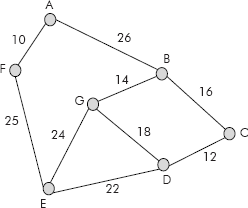
Fig. 8.29 A connected undirected grap
The sorted list of edges in increasing order of their weight is given below:
Edge |
Weight |
A–F |
10 |
C–D |
12 |
B–G |
14 |
B–C |
16 |
D–G |
18 |
D–E |
22 |
E–G |
24 |
E–F |
25 |
A–B |
26 |
Now add the edges starting from shortest edge in sequence from A–F to A–B. The step by step creation of the spanning tree is given in Figure 8.30 (Steps 1–6)
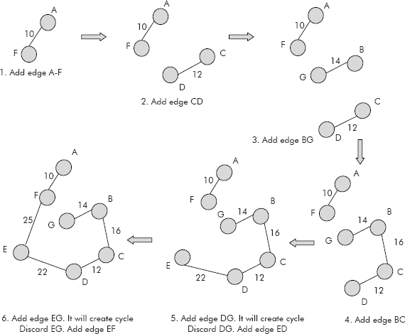
Fig. 8.30 Creation of spanning tree
Having obtained an MST, we are now in a position to appreciate the algorithm proposed by Kruskal as given below:
| Input: | T: An empty spanning tree |
| E: Set of edges | |
| N: Number of nodes in a connected undirected graph |
Kruskal’s algorithm MST()
{
Step 1. sort the edges contained in E in ascending order of their weighs
     2. count = 0
     3. pick an edge of lowest weight from E. Delete it from E
     4. add the edge into T if it does not create a cycle else discard
        it and repeat step 3
     5. count = count +1
     6. if (count < N-1) && E not empty repeat steps 2-5
     7. if T contains less than n-1 edges and E is empty report no spanning tree is possible. Stop.
     8. return T.
)
Example 6: Find the minimum spanning tree for the graph given in Figure 8.31 using Kruskal’s algorithm.
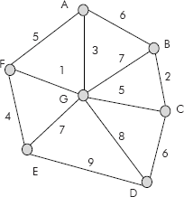
Fig. 8.31 A connected undirected graph
Solution: The sorted list of edges in increasing order of their weight is given below:
Edge |
Weight |
F–G |
1 |
B–C |
2 |
A–G |
3 |
E–F |
4 |
A–F |
5 |
C–G |
5 |
A–B |
6 |
C–D |
6 |
B–G |
7 |
E–G |
7 |
D–G |
8 |
D–E |
9 |
Now add the edges starting from shortest edge in sequence from F–G to D–E. The step by step creation of the spanning tree is given in Figure 8.32 (Steps 1–6)
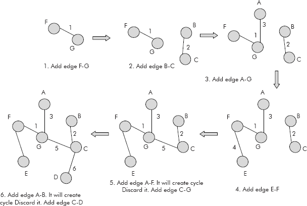
Fig. 8.32 Creation of spanning tree
Prim’s algorithm
In this algorithm the spanning tree is grown in stages. A vertex is chosen at random and included as the first vertex of the tree. Thereafter a vertex from remaining vertices is so chosen that it has a smallest edge to a vertex present on the tree. The selected vertex is added to the tree. This process of addition of vertices is repeated till all vertices are included in the tree. Thus at given moment, there are two set of vertices: T—a set of vertices already included in the tree, and E—another set of remaining vertices. The algorithm for this procedure is given below
| Input: | T: An empty spanning tree |
| E: Empty set of edges | |
| N: Number of nodes in a connected undirected graph |
  Algorithm Prim()
  {
    Step 1. Take random node v add it to T. Add adjacent nodes of v to E
         2. while ( number of nodes in T < N)
         { 2.1 if E is empty then report no spanning tree is possible.
             Stop.
           2.3 for a node x of T choose node y such that the edge (x,y) has lowest cost
           2.4 if node y is in T then discard the edge (x,y) and repeat step 2
           2.5 add the node y and the edge (x,y) to T.
           2.6 delete (x,y) from E.
           2.7 add the adjacent nodes of y to E.
          }
         3. return
 }
It may be noted that the implementation of this algorithm would require the adjacency matrix representation of a graph whose MST is to be generated.
Let us consider the graph of Figure 8.31. The adjacency matrix of the graph is given in Figure 8.33.
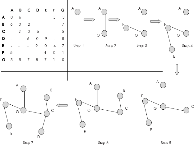
Fig. 8.33 The adjacency matrix and the diferent steps of obtaining MST
Let us now construct the MST from the adjacency matrix given in Figure 8.33. Let us pick A as the starting vertex. The nearest neighbour to A is found by searching the smallest entry (other than 0) in its row. Since 3 is the smallest entry, G becomes its nearest neighbour. Add G to the sub graph as edge AG (see Figure 8.33). The nearest neighbour to sub graph A–G is F as it has the smallest entry i.e. 1. Since by adding F, no cycle is formed then it is added to the sub-graph. Now closest to A–G–F is the vertex E. It is added to the subgraph as it does form a cycle. Similarly edges G–C, C–B, and C–D are added to obtain the complete MST. The step by step creation of MST is shown in Figure 8.33.
8.4.5 Shortest path problem
The communication and transport networks are represented using graphs. Most of the time one is interested to traverse a network from a source to destination by a shortest path. Foe example, how to travel from Delhi to Puttaparthy in Andhra Pradesh? What are the possible routes and which one is the shortest? Similarly, through which route to send a data packet from a node across a computer network to a destination node? Many algorithms have been proposed in this regard but the most important algorithms are Warshall’s algorithm, Floyd’s algorithm, and Dijkstra’s algorithm.
8.4.5.1 Warshall’s Algorithm
This algorithm computes a path matrix from an adjacency matrix A.
The path matrix has the following property:
![]()
Note: The path can be of length one or more
The path matrix is also called the transitive closure of A i.e. if path [i][k] and Path [k][j] exist then path [1][j] also exists.
We have already introduced this concept in Section 8.3.1 vide Property 3 wherein it was stated that “For a given adjacency matrix A, the element Aij of matrix Ak (kth power of A) gives the number of paths of length k from vertex vi to vj”. Therefore, the transitive closure of an adjacency matrix A is given by the following expression:
Path = A + A1 + A2 + … + An
The above method is compute intensive as it requires a series of matrix multiplication operations to obtain a path matrix.
Example 7: Compute the transitive closure of the graph given in Figure 8.34.
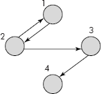
Fig. 8.34
Solution: The step wise computation of the transitive closure of the graph is given in Figure 8.35.
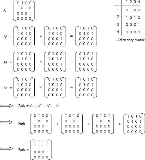
Fig. 8.35 Transitive closure of a graph
Warshall gave a simpler method to obtain a path or reachability matrix of a directed graph (diagraph) with the help of only AND or OR Boolean operators. For example, it determines whether a path form vertex vi to vj through vk exists or not by the following formula
Path [i][j] = Path [i][j] V ([i][k] Λ Path [k][j])
Thus, Warshall’s algorithm also computes the transitive closure of an adjacency matrix of a diagraph.
The algorithm is given below:
Input: Adjacency matrix A[][] of order n*n
Path Matrix Path[][] of order n*n, initially empty
Algorithm Warshall()
{ /* copy A to Path */
  for (i = 1; i < = n; i++)
  {
    for ( j = 1; j < = n; j++)
    {
      Path [i][j] = A[i][j];
    }
  }
                   /* Find path from vi to vj through vk */
  for (k = 1; k <= n; k++)
  { for (i = 1; i < = n; i++)
    {
      for (j = 1; j < = n; j++)
      { Path [i][j] = Path[i][j] || (Path [i][k] && Path [k][j]);
      }
    }
  }
    return Path;
}
Example 8: Apply Warshall’s on the graph given in Figure 8.34 to obtain its path matrix
Solution: The step by step of the trace of Warshall’s algorithm is given in Figure 8.36.
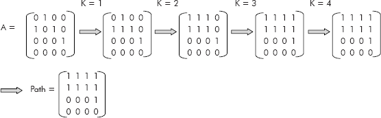
Fig. 8.36
8.4.5.2 Floyd’s Algorithm
The Floyd’s algorithm is almost same as Warshall’s algorithm. The Warshal’s algorithm establishes as to whether a path between vertices vi and vj exists or not? The Floyd’s algorithm finds a shortest path between every pair of vertices of a weighted graph. It uses the following data structures:
- A cost matrix, Cost [][] as defined below:
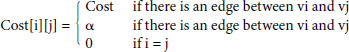
- A distance matrix Dist[][] wherein an entry D[i][j] is the distance of the shortest path from vertex vi to vj.
In fact, for given vertices vi and vj, it finds out a path from vi to vj through vk. If vi–vk–vj path is shorter than the direct path from vi to vj then vi–vk–vj is selected. It uses the following formula (similar to Warshall):
Dist [i][j] = min ( Dist[i][j], ( Dist[i][k] + Dist [k][j])
The algorithm is given below:
Algorithm Floyd ()
{
  for (i = 1; i <= n; i++)
    for (j = 1; j <= n; j++)
      Dist[i][j] = Cost[i][j]; /* copy cost matrix to distance matrix */
  for ( k = 1; k <= n; k++)
  { for (i = 1; i <= n; i++)
     { for (j = 1; j <= n; j++)
        Dist[i][j] = min ( Dist[i][j] , ( Dist[i][k] + Dist [k][j];
     }
  }
}
Example 9: For the weighted graph given in Figure 8.37, find all pairs shortest paths using Floyd’s algorithm.
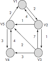
Fig. 8.37
Solution: The cost matrix and the step by step of the trace of Floyd’s algorithm is given in Figure 8.38.
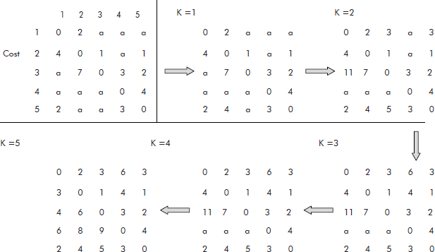
Fig. 8.38
8.4.5.3 Dijkstra’s Algorithm
This algorithm finds the shortest paths from a certain vertex to all vertices in the network. It is also known as single source shortest path problem. For a given weighted graph G = (V, E), one of the vertices v0 is designated as a source. The source vertex v0 is placed on a set S with its shortest path taken as zero. Where the set S contains those vertices whose shortest paths are known. Now iteratively, a vertex (say vi) from remaining vertices is added to the set S such that its path is shortest from the source. In fact this shortest path from v0 to vi passes only through the vertices present in set S. The process stops as soon as all the vertices are added to the set S.
The dijkstra algorithm uses following data structures:
- A vector called Visited[]. It contains the vertices which have been visited. The vertices are numbered from 1 to N. Where N is number of vertices in the graph. Initially Visited is initialized as zeros. As soon as a vertex i is visited (i.e. its shortest distance is found) Visited[i] is set to 1.
- A two dimensional matrix Cost[][]. An entry Cost[i][j] contains the cost of an edge (i, j). If there is no edge between vertices i and j then cost[i][j] contains a very large quantity (say 9999).
- A vector dist[]. An entry dist[i] contains the shortest distance of ith vertex from the starting vertex v1.
- A vector S contains those vertices whose shortest paths are now known.
The algorithm is given below:
Algorithm dijkstra ()
{
  S[1] =1; Visited [1] = 1; dist[1] =0; /* Initialize. Place v1 on S */
  for ( i = 2; i <= N; i++; )
  {
    Visited [i] = 0;
    dist [i] = cost [1][i]
  }
for (i = 2; i <= N; i++;)
       /* Find vertex with minimum cost and its number stored in pos */
{
  min = 9999; pos = -1;

  for ( j = 2; j <= N; j++)
  {
    if (visited [j] = 0 && dist[j] < min )
    {
      pos = j;
      min = dist[j];
    }
  }
                  /* Add the vertex (i.e. pos)
    visited [pos] = 1; S[i] = pos;
/* for each vertex adjacent to pos, update distances */
for ( k = 2; k <=N; k++)
  {
    if (visited [k] == 0)
      if ( dist (pos) + cost [pos][k] < dist [k])
        dist [k] = dist (pos) + cost [pos][k];
  }
 }
Consider the graph given in Figure 8.39.
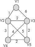
Fig. 8.39 An undirected weighted graph
The corresponding cost matrix and the stepwise construction of shortest cost of all vertices with re-spect to vertex V1 is given in Figure 8.40.
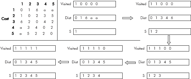
Fig. 8.40 Cost matrix and different steps of Dijkstra’s algorithm
Example 10: For the graph given in Figure 8.41 , find the shortest path from vertex A to all the remaining verices.
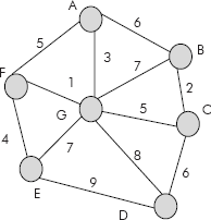
Fig. 8.41
Solution: Let us number the vertices A–G as 1–7. The corresponding cost matrix and the stepwise construction of shortest cost of all vertices with respect to vertex 1 (i.e. A) is given in Figure 8.42.
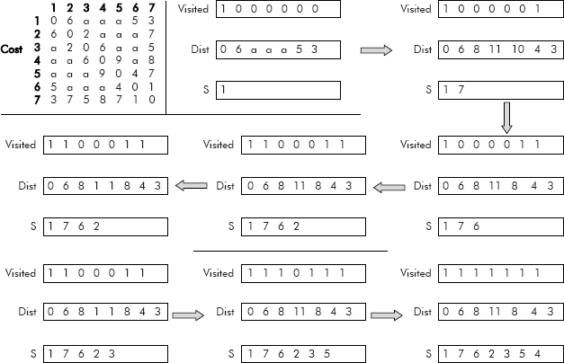
Fig. 8.42 Cost matrix and different steps of Dijkstra’s algorithm
8.5 APPLICATIONS OF GRAPHS
There are numerous applications of graphs. Some of the important applications are as follows:
- Model of www: The model of world wide web (www) can be represented by a graph (directed) wherein nodes denote the documents, papers, articles, etc. and the edges represent the outgoing hyperlinks between them as shown in Figure 8.43.
It may be noted that a page on site S1 has a link to page on site S4. The pages on S4 refer to pages on S2 and S3, and so on. This hyperlink structure is the basis of the web structure similar to the web created by a spider and, hence, the name world wide web.
- Resource allocation graph: In order to detect and avoid deadlocks, the operating system maintains a resource allocation graph for processes that are active in the system. In this graph, the processes are represented as rectangles and resources as circles. Number of small circles within a resource node indicates the number of instances of that resource available to the system. An edge from a process P to a resource R, denoted by (P, R), is called a request edge. An edge from a resource R to a process P, denoted by (R, P), is called an allocation edge as shown in Figure 8.44.
It may be noted from the resource allocation graph of Figure 8.27 that the process P1 has been allocated one instance of resource R1 and is requesting for an instance of resource R2. Similarly, P2 is holding an instance of both R1 and R2. P3 is holding an instance of R2 and is asking for an instance of R1. The edge (R1, P1) is an allocation edge whereas the edge (P1, R2) is a request edge.
An operating system maintains the resource allocation graph of this kind and monitors it from time to time for detection and avoidance of deadlock situations in the system.
- Colouring of maps: Colouring of maps is an interesting problem wherein it is desired that a map has to be coloured in such a fashion that no two adjacent countries or regions have the same colour. The constraint is to use minimum number of colours. A map (see Figure 8.45) can be represented as a graph wherein a node represents a region and an edge between two regions denote that the two regions are adjacent.
- Scene graphs: The contents of a visual scene are also managed by using graph data structure. Virtual reality modelling language (VRML) supports scene graph programming model. This model is used by MPEG-4 to represent multimedia scene composition.
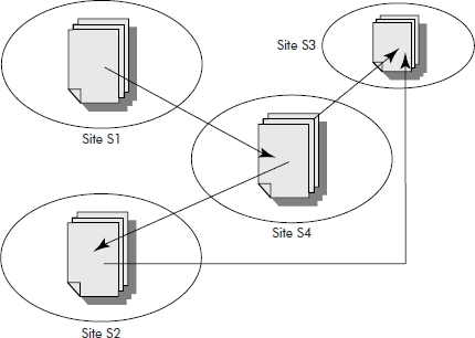
Fig. 8.43 The graphic representation of www
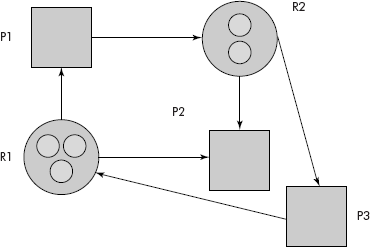
Fig. 8.44 A resource allocation graph
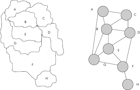
Fig. 8.45 The graphic representation of a map
A scene graph comprises nodes and edges wherein a node represents objects of the scene and the edges define the relationship between the objects. The root node called parent is the entry point. Every other node in the scene graph has a parent leading to an acyclic graph or a tree like structure as shown in Figure 8.46.
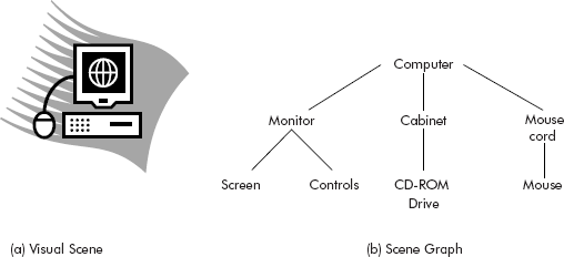
Fig. 8.46 A scene graph for a visual scene
For more reading on scene graphs, the reader may refer to the paper “Understanding Scene Graphs” by Aeron E. Walsh, chairman of Mantis development at Boston College.
Besides above, the other popular applications of graphs cited in books are:
- Shortest path problem
- Spanning trees
- Binary decision graph
- Topological sorting of a graph
EXERCISES
- Explain the following graph theory terms:
- Node
- Edge
- Directed graph
- Undirected graph
- Connected graph
- Disconnected graph
- What is a graph and how is it useful?
- Draw a directed graph with five vertices and seven edges. Exactly one of the edges should be a loop, and should not have any multiple edges.
- Draw an undirected graph with five edges and four vertices. The vertices should be called v1, v2, v3 and v4 and there must be a path of length three from v1 to v4.
- Draw the directed graph that corresponds to the following adjacency matrix:
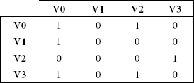
Also, write down the adjacency list corresponding to the graph.
- Write a ‘C’ function to compute the indegree and outdegree of a vertex of a directed graph when the graph is represented by an adjacency list.
- Write a program in ‘C’ to implement graph using adjacency matrix and perform the following operations:
- Depth First Search
- Breadth First Search
- Consider a graph representing an airline’s network: each node represents an airport, and each edge represents the existence of a direct flight between two airports. Suppose that you are required to write a program that uses this graph to find a flight route from airport p to airport q. Would you use breadth first search or depth first search? Explain your answer.
- Write the adjacency matrix of the graph shown in figure below. Does the graph have a cycle? If it has, indicate all the cycles.
- Writea function that inserts an edge into a undirected graph represented using an adjacency matrix.
- Write a function that inserts an edge into a directed graph represented using an adjacency matrix.
- Write a function that deletes an edge from a directed graph represented using an adjacency matrix.
- Write a function that deletes an edge from an undirected graph represented using an adjacency matrix.
- Find the minimum spanning tree for the graph given in Figure 8.39.
- Write the Warshall’s algorithm.
- Write the Dijkstra’s algorithm.
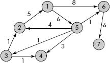
Fig. 8.47