
Chapter 10
Advanced Data Structures
CHAPTER OUTLINE
10.1 AVL TREES
During the discussion on binary search trees (BST) in Chapter 7, it was appreciated that BST is an excellent tool for fast search operations. It was also highlighted that if the data input to BST is not properly planned, then there is every likelihood that the BST may end up in a skewed binary tree or at least a lopsided binary tree wherein one subtree has more height than the other subtree. Consider the data given below:
Cat Family = {Lion, Tiger, Puma, Cheetah, Jaguar, Leopard, Cat, Panther, Cougar, Lynx, Ocelot}
This data can be provided in any combination and the resultant BSTs would be different from each other depending upon the pattern of input. Some of the possible BSTs produced from the above data are shown in Figure 10.1.
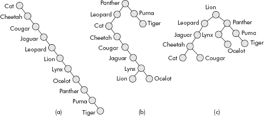
Fig. 10.1 BSTs produced from same data provided in different combinations
It may be noted that the BST of Figure 10.1 (a) is a skewed binary tree and the search within such a data structure would amount to a linear search. The BST of Figure 10.1 (b) is heavily lopsided towards left whereas the BST of Figure 10.1 (c) is somewhat balanced and may lead to a comparatively faster search. If the data is better planned, then definitely an almost balanced BST can be obtained. But the planning can only be done when the data is already with us and is suitably arranged before creating the BST out of it. However, in many applications such as ‘symbol processing’ in compilers, the data is dynamic and unpredictable and, therefore, creation of a balanced BST is a remote possibility. Hence, the need to develop a technique that maintains a balance between the heights of left and right subtrees of a binary tree has always been felt; the major aim being that whatever may be the order of insertion of nodes, the balance between the subtrees is maintained.
A height balanced binary tree was developed by Adelson-Velenskii and Landis, Russian researchers, in 1962 which is popularly known as an ‘AVL Tree’. The AVL Tree assumes the following basic subdefinitions:
- The height of a tree is defined as the length of the longest path from the root node of the tree to one of its leaf nodes.
- The balance factor (BF) is defined as given below:
BF = height of left subtree (HL) – height of right subtree (HR)
With the above subdefinitions, the AVL Tree is defined as a balanced binary search tree if all its nodes have balance factor (BF) equal to –1, 0, or 1.
In simple words we can say that in AVL Tree, the height of two subtrees of a node differs by at most one. Consider the trees given in Figure 10.2.
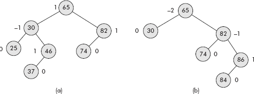
Fig. 10.2 The binary search trees with BF labelled at each node
It may be noted that in Figure 10.2 (a), all nodes have BF within the range, i.e. –1, 0, or 1. Therefore, it is an AVL Tree. However, the root of graph in Figure 10.2 (b) has BF equal to −2, which is a violation of the rule and hence the tree is not AVL.
Note: A complete binary search tree is always height balanced but a height balanced tree may or may not be a complete binary tree.
The height of a binary tree can be computed by the following simple steps:
- If a child is NULL then its height is 0.
- The height of a tree is = 1 + max (height of left subtree, height of right subtree)
Based on the above steps, the following algorithm has been developed to compute the height of a general binary tree:
Algorithm compHeight (Tree)
   {
     if (Tree == NULL)
      {height = 0; return height}
     hl = compHeight (leftChild (Tree));
     hr = compHeight (rightChild (Tree));
     if (hl >= hr) height = hl + 1;
     else
       height = hr + 1;
     return height;
 }
The following operations can be performed on an AVL Tree:
- Searching an AVL Tree.
- Inserting a node in an AVL Tree.
- Deleting a node from an AVL Tree.
10.1.1 Searching an AVL Tree
An AVL Tree can be searched for a key K by visiting nodes starting from root. The visited node is checked for the presence of K. If found, then the search stops otherwise if value of K is less than the key value of visited node, then the left subtree is searched else the right subtree is searched. The algorithm for AVL search is given below:
Algorithm searchAVL (Tree, K)
   {
     if (DATA (Tree) == K)
       {prompt " Search successful" ; Stop;}
     if (DATA (Tree) < K)
       searchAVL (leftChild (Tree), K);
     else
       searchAVL (rightChild(Tree), K);
 }
The search for key (K = 37) will follow the path as given in Figure 10.3.
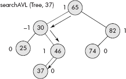
Fig. 10.3 Search for a key within an AVL tree
10.1.2 Inserting a Node in an AVL Tree
Whenever a node is inserted into a subtree which is full and whose height is already 1 more than its sibling, then the subtree becomes unbalanced. This imbalance in a subtree ultimately leads to imbalance of whole of the tree as shown in Figure 10.4. An insertion of node ‘50’ has caused an imbalance in the tree. The nearest ancestor whose BF has become ±2 is called a pivot. The node 30 is the pivot in the unbalanced tree of Figure 10.4.
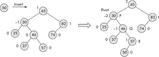
Fig. 10.4 An insertion into a full subtree
The imbalance can be removed by carefully rearranging the nodes of the tree. For instance, the zone of imbalance in the tree is the left subtree with root node 30 (say Node P). Within this subtree, the imbalance is in right subtree with root node 46 (say Node Q). The closest node to the inserted node is 57. Call this node as R. A point worth noting is that P, Q, and R are numbers and can be rearranged as per binary search rule, i.e., the smallest becomes the left child, the largest as the right child and the middle one becomes the root. This rearrangement can eliminate the imbalance in the section as shown in Figure 10.5.
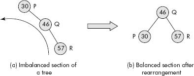
Fig. 10.5 The rearrangement of nodes
It may be noted that imbalanced section of the tree has been rotated to left to balance the subtree. The rotation of a subtree in an AVL Tree is called an AVL rotation. Depending upon, in which side of the pivot a node is inserted, there are four possible types of AVL rotations as discussed in following sections.
10.1.2.1 Insertion of a Node in the Left Subtree of the Left Child of the Pivot
In this case, when a node in an AVL Tree is inserted in the left subtree of the left child (say LL) of the pivot then the imbal-ance occurs as shown in Figure 10.6 (a).
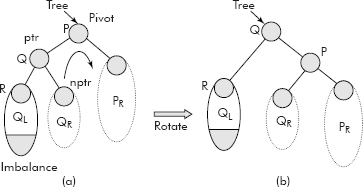
Fig. 10.6 AVL rotation towards right
It may be noted that in this case, after the rotation, the pivot P has become the right child, Q has become the root. QR, the right child of Q has become the left child of P. The QL, the left child of Q remains intact.
The algorithm for this rotation is given below:
/* The Tree points to the Pivot */

Algorithm rotateLL (Tree)
  {
    ptr = leftChild (Tree); /* point ptr to Q */
    nptr = rightChild (ptr); /* point nptr to right child of Q */
    rightChild (ptr) = Tree; /* attach P as right child of Q */
    leftChild (Tree) = nptr; /* attach right child of Q as left child of P */
    Tree = ptr; /* Q becomes the root */
    return Tree;
  }
Consider the AVL Tree given in Figure 10.7 (a). The tree has become imbalanced after the insertion of 12 [see Figure 10.7 (b)].
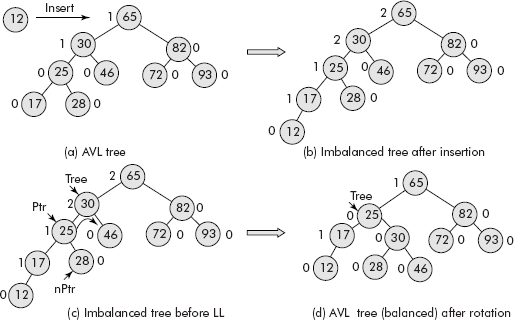
Fig. 10.7 The AVL rotation (LL)
Figure 10.7c shows the application of pointers on the nodes of the tree as per the AVL rotation. Figure 10.7 (d) shows the final AVL Tree (height balanced) after the AVL rotation, i.e., after the rearrangement of nodes.
10.1.2.2 Insertion of a Node in the Right Subtree of the Right Child of the Pivot
In this case, when a node in an AVL Tree is inserted in the right subtree of the right child (say RR) of the pivot then the imbalance occurs as shown in Figure 10.8 (a).
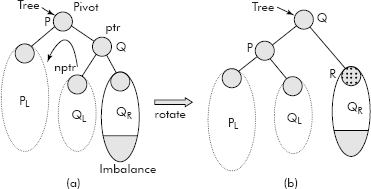
Fig. 10.8 AVL rotation towards left
It may be noted that in this case, after the rotation, the pivot P has become the left child, Q has be-come the root. QL, the left child of Q (i.e, QL) has become the right child of P. The QR, the right child of Q remains intact.
The algorithm for this rotation is given below:
 /* The Tree points to the Pivot */

 Algorithm rotateRR (Tree)
   {
     ptr = rightChild (Tree); /* point ptr to Q */
     nptr = leftChild (ptr); /* point nptr to left child of Q */
     leftChild (ptr) = Tree; /* attach P as left child of Q */
     rightChild (Tree) = nptr; /* attach left child of Q as right child of P */
     Tree = ptr; /* Q becomes the root */
     return Tree;
   }
Consider the AVL Tree given in Figure 10.9 (a). The tree has become imbalanced after the inser-tion of 100 (see Figure 10.9 (b)).
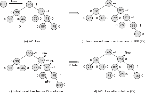
Fig. 10.9 The AVL rotation (RR)
Figure 10.9 (c) shows the application of pointers on the nodes of the tree as per the AVL rotation. Figure 10.9 (d) shows the final AVL Tree (height balanced) after the AVL rotation, i.e., after the rearrangement of nodes.
10.1.2.3 Insertion of a Node in the Right Subtree of the Left Child of the Pivot
In this case, when a node in an AVL Tree is inserted in the right subtree of the left child (say LR) of the pivot then the imbalance occurs as shown in Figure 10.10 (a).
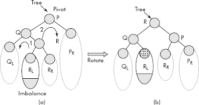
Fig. 10.10 The double rotation Left-Right (LR)
This case requires two rotations: rotation 1 and rotation 2.
Rotation 1: In this rotation, the left child of R becomes the right child of Q and R becomes the left child of P. Q becomes the left child of R. The right child of R remains intact.
Rotation 2: In this rotation, the right child of R becomes the left child of P. R becomes the root. P becomes the right child of R.
The final balance tree after the double rotation is shown in Figure 10.10 (b).
The algorithm for this double rotation is given below:
 /* The Tree points to the Pivot */

 Algorithm rotate LR (Tree)
   {
     ptr = leftChild (Tree); /* point ptr to Q */
     rotateRR (ptr); /* perform the first rotation */
     ptr = leftChild (Tree); /* point ptr to R */
     rotate LL (ptr);
   }
The trace of the above algorithm is shown in Figure 10.11 wherein the AVL Tree has become imbalanced because of insertion of node 50 in the right subtree of left child of pivot [see Figures 10.11 (a) and (b)].
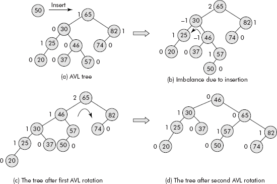
Fig. 10.11 The trace of double rotation on an imbalanced AVL tree
After the double rotation, the tree has again become height balanced as shown in Figures 10.11 (c) and (d).
10.1.2.4 Insertion of a Node in the Left Subtree of the Right Child of the Pivot
In this case, when a node in an AVL Tree is inserted in the left subtree of the right child (say LR) of the pivot then the imbalance occurs as shown in Figure 10.12 (a).
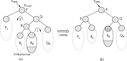
Fig. 10.12 The double rotation Right-Left (RL)
This case also requires two rotations: rotation 1 and rotation 2.
Rotation 1: In this rotation, the right child of R becomes the left child of Q and R becomes the right child of P. Q becomes the right child of R. The left child of R remains intact.
Rotation 2: In this rotation, the left child of R becomes the right child of P. R becomes the root. P becomes the left child of R.
The final balance tree after the double rotation is shown in Figure 10.12 (b).
Following is the algorithm for this double rotation:
 /* The Tree points to the Pivot */

 Algorithm rotate RL (Tree)
   {
     ptr = rightChild (Tree); /* point ptr to Q */
     rotateLL (ptr); /* perform the first rotation */
     ptr = rightChild (Tree); /* point ptr to R */
     rotateRR (ptr);
   }
The trace of the above algorithm is shown in Fig. 10.13 wherein the AVL tree has become imbalanced because of insertion of node 92 the left subtree of right child of pivot (See Fig. 10.13(a), (b)). After the double rotation, the tree has again become height balanced as shown in Fig. 10.13(c), (d).
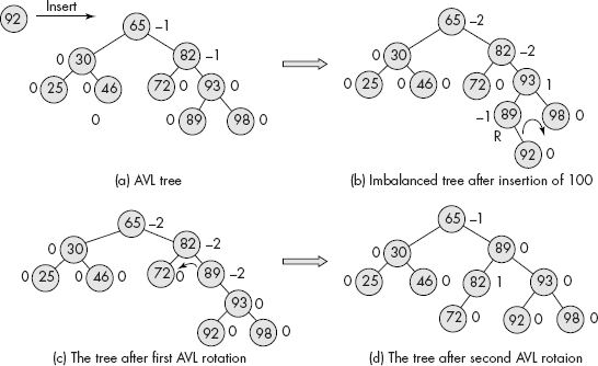
Fig. 10.13 The trace of double rotation on an imbalanced AVL tree
10.2 SETS
A set is an unordered collection of homogeneous elements. Each element occurs at most once with the following associated properties:
- All elements belong to the Universe. The Universe is defined as “all potential elements of set”.
- An element is either a member of the set or not.
- The elements are unordered.
Some examples of sets are given below.
Cat_ Family = {Lion, Tiger, Puma, Cheetah, Jaguar, Leopard, Cat, Panther, Cougar, Lynx, Ocelot}
Fruits = {mango, orange, banana, grapes, apple, guava, peach}
LAN = {Comp, Mech, Elect, Civil, Accts, Estb, Mngmt, Hostel}
Note: The LAN is a set of nodes of a local area network of an educational institute spread over various departments like computer engineering, mechanical engineering, electrical engineering, etc.
The basic terminology associated with sets is given below:
- Null set: If a set does not contain any element, then the set is called empty or null set. It is represented by Φ.
- Subset: If all elements of a set S1 are contained in set S2, then S1 is called a subset of S2. It is denoted by S1 ⊆ S2.
Example: The set of big_Cat = {Lion, Tiger, Panther, Cheetah, Jaguar} is a subset of the set of Cat_Family.
- Union of sets: The union of two sets S1 and S2 is obtained by collecting all members of either set without duplicate entries. This is represented by S1 ⋃ S2.
Example: If S1 = {1, 3, 4}, S2 = {4, 5, 6, 7, 8}, then S1 ⋃S2 = {1, 3, 4, 5, 6, 7, 8}.
- Intersection of sets: The intersection of two sets S1 and S2 is obtained by collecting common elements of S1 and S2. This is represented by S1 ∩ S2.
Example: If S1 = {1, 3, 4}, S2 = {4, 5, 6, 7, 8}, then S1 ∩ S2 = {4}.
- Disjoint sets: If two sets S1 and S2 do not have any common elements, then the sets are called disjoint sets, i.e., S1 ∩ S2 = Φ.
Example: S1 = {1, 3}, S2 = {4, 5, 6, 7, 8} are disjoint sets.
- Cardinality: Cardinality of a set is defined as the number of unique elements present in the set. The cardinality of a set S is represented as |S|.
Example: If S1 = {1, 3, 4}, S2 = {4, 5, 6, 7, 8}, then |S1| = 3 and |S2| = 5.
- Equality of sets: If S1 is subset of S2 and S2 is subset of S1, then S1 and S2 are equal sets. This means that all elements of S1 are present in S2 and all elements of S2 are present in S1.The equality is represented as S1 ⊆ S2.
Example: If S1 = {1, 3, 4}, S2 = {3, 1, 4}, then S1 ≡ S2.
- Difference of sets: Given two sets S1 and S2, the difference S1 – S2 is defined as the set having all the elements which are in S1 but not in S2.
Example: If S1 = {1, 3, 4}, S2 = {3, 2, 5}, then S1 – S2 = {1, 4}.
The graphic representation of various operations related to sets is shown in Figure 10.14.
- Partition: It is a collection of disjoint sets belonging to same Universe. Thus, the union of all the disjoint sets of a partition would comprise the Universe.
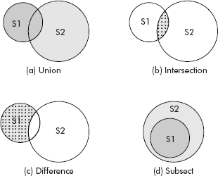
Fig. 10.14 Various set operations
10.2.1 Representation of Sets
A set can be represented by the following methods:
- List representation
- Hash table representation.
- Bit vector representation
- Tree representation
List and hash table representations are more popular methods as compared to other methods. A brief discussion on list and hash table representations is given in following sections.
10.2.1.1 List Representation
A set can be very comfortably represented using a linear linked list. For example, the set of fruits can be represented as shown in Figure 10.15.
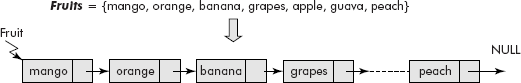
Fig. 10.15 The list representation of a set
Since the set is an unordered collection of elements, linked list is the most suitable representation for the sets because elements can be dynamically added or deleted from a set.
10.2.1.2 Hash Table Representation
Hash table representation of a set is also a version of linked representation. A hash table consists of storage locations called buckets. The size of a bucket is arbitrary, i.e., it can hold any number of elements as it stores them into a linked list.
Consider the following set:
Tokens = {126, 235, 100, 317, 68, 129, 39, 423, 561, 222, 986}
Let us store the above set in a hash table of five buckets with hash function as given below:
H(K) = K mod 5
Where, K is an element;
H(K) gives the bucket number in which the element K is to be stored.
The arrangement is shown in Figure 10.16.
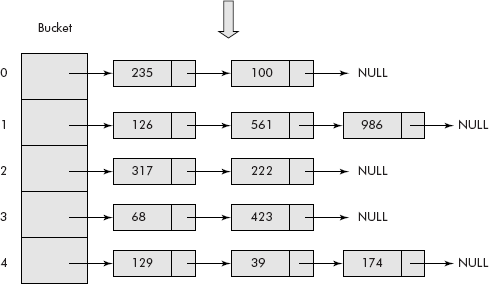
Fig. 10.16 Hash table representation of a set
Tokens = {126, 235, 100, 317, 68, 129, 39, 423, 561, 222, 986}
It may be noted that each bucket is having a linked list consisting of nodes containing a group of elements from the set.
10.2.2 Operations on Sets
The following operations can be defined on sets:
- Union
- Intersection
- Difference
- Equality
A brief discussion on each operation is given in the sections that follow.
10.2.2.1 Union of Sets
As per the definition, given two sets S1 and S2, the union of two sets is obtained by collecting all the members of either set without duplicate entries. Let us assume that the sets have been represented using lists as shown in Figure 10.17. The union set S3 of S1 and S2 has been obtained by the following steps:

Fig. 10.17 Union of sets
- Copy the list S1 to S3.
- For each element of S2, check if it is membero of S1 or not and if it is not present in S1 then attach it at the end of S3.
The algorithm for union of two sets S1 and S2 is given below:
/* This algorithm uses two functions: copy() and ifMember(). The copy ()
   function is used to copy a set to another empty set (say S1 to S3). The
   ifMember function is employed to test the membership of an element in a given set */

 Algorithm unionOfSets (S1, S2)
  {
    S3 = Null;
    S3 = copy (S1, S3, last); /* copy Set S1 to S3 */
    ptr = S2;
    while (ptr != Null)
    {
      Res = ifMember (ptr, S1); /* Check membership of ptr in S1 */
      if (Res == 0)
      { /* if the node of S2 is not member of S1 */

      nptr = new node;
      DATA (nptr) = DATA (ptr)
      NEXT (nptr) = NULL;
      NEXT (last) = nptr;
      last = nptr;
    }
    ptr = Next (ptr);
  }
  return S3;
}

/* This function is used to copy a set to another empty set, i.e., Set1
   to Set3 */

Algorithm copy (S1, S3)
  {
    ptr = S1;
    back = S3;
    ahead = Null;
    while (ptr != Null)
    {  ahead = new node;
       DATA (ahead) = DATA (ptr);
       NEXT (ahead) = Null;
       if (back == Null) /* first entry into S3 i.e. S3 is also Null */
       {
         back = ahead;
         S3 = ahead;
       }
       else
       {
         NEXT (back) = ahead;
         back = ahead;
       }
       ptr = NEXT (ptr);
     }
     return S3;
  }

  /* This function is employed to test the membership of an element by pointed ptr, in a given set S */

Algorithm ifMember (ptr, S)
  {
    Flag = 0;
    nptr = S;
    while (nptr != Null)
    {
   if (DATA (ptr) = = DATA (nptr))
   {
      Flag = 1;
      break;
   }
   nptr = NEXT (nptr);
  }
  return Flag;
 }
10.2.2.2 Intersection of Sets
As per the definition, given two sets S1 and S2, the intersection of two sets is obtained by collecting all the common members of both the sets. Let’s assume that the sets have been rep-resented using lists as shown in Figure 10.18. The intersection set S3 of S1 and S2 has been obtained by the following steps:
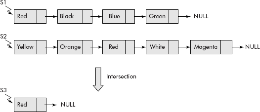
Fig. 10.18 Intersection of sets
- Initialize S3 to Null;
- last = S3;
- For each element of S2, check if it is member of S1 or not and if it is present in S1 then attach it at the end of S3.
The algorithm for intersection of two sets S1 and S2 is given below:
/* This algorithm uses the function ifMember() which tests the membership of an element in a given set */

Algorithm intersectionOfSets (S1, S2)
  {
    S3 = Null;
    last = S3;
    ptr = S2;
    while (ptr != Null)
  {
      Res = ifMember (ptr, S1); /* Check membership of ptr in S1 */

     if (Res == 1)
     { /* if the node of S2 is member of S1 */
       nptr = new node;
       DATA (nptr) = DATA (ptr)
       NEXT (nptr) = NULL;
       If (last == Null) /* S3 is empty and it is first entry */
       {
           last = nptr;
           S3 = last;
       }
       else
       {
       NEXT (last) = nptr;
       last = nptr;
     }
   }
   ptr = Next (ptr);
  }
  return S3;
 }
Note: The ifMember() function is already defined in the previous section.
10.2.2.3 Difference of Sets
As per the definition, given two sets S1 and S2, the difference S1 − S2 is obtained by collecting all the elements which are in S1 but not in S2. Let us assume that the sets have been represented using lists as shown in Figure 10.19. The difference set S3, i.e., S1 − S2 has been obtained by the following steps:
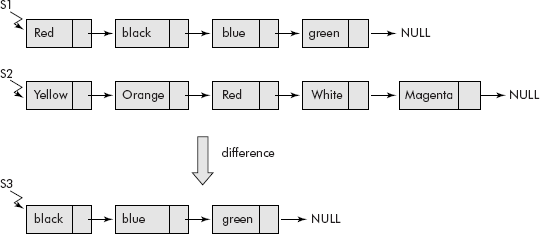
Fig. 10.19 Diference of sets
- Initialize S3 to Null;
- last = Null;
- For each element of S1, check if it is a member of S2 or not and if it is not present in S2 then attach it at the end of S3.
The algorithm for difference of two sets S1 and S2 is given below:
/* This algorithm uses the function ifMember() which tests the membership of an element in a given set */

 Algorithm differenceOfSets (S1, S2)
  {
     S3 = Null;
     last = S3;
     ptr = S1;
     while (ptr != Null)
      {
       Res = ifMember (ptr, S2); /* Check membership of ptr in S2 */
       if (Res == 0)
       {   /* if the node of S1 is not member of S2 */
          nptr = new node;
          DATA (nptr) = DATA (ptr)
          NEXT (nptr) = NULL;
          If (last == Null) /* S3 is empty and it is first entry */
         {
              last = nptr;
              S3 = last;
         }
         else
         {
             NEXT (last) = nptr;
             last = nptr;
       }
     }
     ptr = Next (ptr);
   }
   return S3;
  }
Note: The ifMember() function is already defined in the previous section.
10.2.2.4 Equality of Sets
As per the definition, given two sets S1 and S2, if S1 is subset of S2 and S2 is subset of S1 then S1 and S2 are equal sets. Let us assume that the sets have been represented using lists. The equality S1 ≡ S2 has been obtained by the following steps:
- For each element of S1, check if it is a member of S2 or not and if it is not present in S2 then report failure.
- For each element of S2, check if it is a member of S1 or not and if it is not present in S1 then report failure.
- If no failure is reported in step1 and step 2, then infer that S1 ≡ S2.
The algorithm for equality of two sets S1 and S2 is given in the following:
/* This algorithm uses the function ifMember() which tests the membership of an element in a given set */

Algorithm equalSets (S1, S2)
  {
    ptr = S1;
    flag = 1;
    while (ptr != Null)
   {
       Res = ifMember (ptr, S2); /* Check membership of ptr in S2 */
       if (Res == 0)
       {flag = 0;
       break;
      }
      ptr = NEXT (ptr);
   }
   if (flag == 0) {prompt "not equal”;  exit ();}
   ptr = S2;
   while (ptr != Null)
   {
      Res = ifMember (ptr, S1); /* Check membership of ptr in S1 */
      if (Res == 0)
      {flag = 0;
      break;
      }
   ptr = NEXT (ptr);
   }
   if (flag == 0) {prompt “not equal”;  exit ();}
   else
                   prompt “Sets equal”;
}
Note: The ifMember() function is already defined in the previous section.
10.2.3 Applications of Sets
There are many applications of sets and a few of them are given below:
- Web linked pages: For each item displayed to user, Google offers a link called “Similar” pages (see Figure 10.20), which is in fact the list of URLs related to that item. This list can be maintained as a set of related pages by using Union operation.
Consider the web pages visited by a user as shown in Figure 10.21.
The arrows between the various pages indicate the link between them. Initially, all pages are stored as singletons in the order of their visit by the users as given below:
{P4}, {P11}, {P7}, {P6}, …… {P5}
Afterwards, the related pages are grouped together by union of the participating singletons as shown below:
- {P4} ⋃ {P7} ⋃ {P11} ⋃ {P9}
- {P6} ⋃ { P12} ⋃ { P4}
- {P5}
We get the following three related partitions, i.e., the disjoint sets:
- P4, P7, P11, P9
- P6, P12, P4
- P5
From the above representation, it can be found as to whether two elements belong to the same set or not. For example, P6 and P12 belong to the same set. A click on page P11 would produce a list of links to P4, P7 and P9, grouped as “Similar” pages to P11.
- Colouring black and white photographs: This is an interesting application in which an old black and white photograph is converted into a coloured one. The method is given below:
- The black and white photograph is digitized, i.e., it is divided into pixels of varying shades of grey, i.e., ranging from white to black.
- Pixels belonging to the same part or component are called equivalent pixels. For example, pixels belonging to eyeballs are equivalent. Similarly, pixels belonging to the shirt of a person are equivalent.
- The equivalence is decided by comparing the grey levels of adjacent pixels.
- In fact, 4 pixels are taken at a time to find the equivalent pixels among the adjacent pixels. This activity is also called 4-pixel square scan.
- The scanning starts from left to right and top to bottom.
- Each pixel is assigned a colour.
- The equivalent pixels are given the same colour.
- If two portions with different coloured pixels meet each other, then it is considered as part of the same component and then both the portions are coloured with the same colour chosen from either of the colours as shown in Figure 10.22.
It may be noted that the equivalence relation between the pixels is obtained through set operations where an equivalence relation R over a set S can be seen as a partitioning of S into disjoint sets.
- Spelling checker: A spelling checker for a document editor is another interesting application of sets, especially the hash table representation. A normal dictionary is maintained using hash table representation of sets. A simple-most dictionary (Dict.) will have 26 buckets because there are 26 alphabets in English language. Similarly, the words of a document (Doc) would also be represented in the same fashion as shown in Figure 10.23. A difference operation Doc – Dict would produce all those words which are in document but not in dictionary, i.e., the misspelled words.
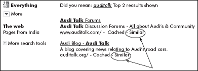
Fig. 10.20 The link to similar URLs
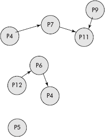
Fig. 10.21 The web pages visited by a user

Fig. 10.22 The colouring of black and white photographs
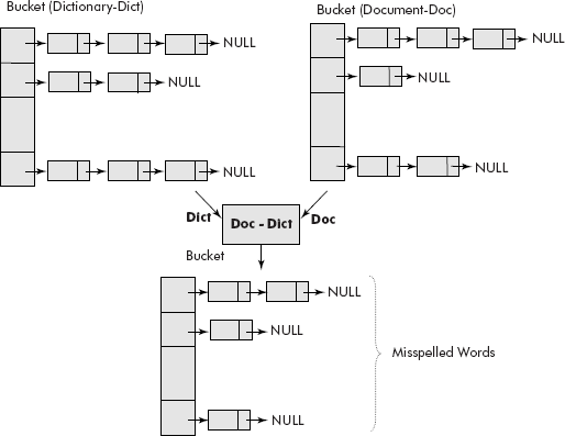
Fig. 10.23 The working of spelling checker
10.3 SKIP LISTS
Search is a very widely used operation on lists. A one-dimensional array is most suitable data structure for a list that does not involve insertion and deletion operations. If the list is unsorted, linear search is used and for a sorted list, binary search is efficient and takes O(log n) operations.
For random input, AVL Trees can be used to search, insert, and delete numbers with time complexity as O(log n). However, the balancing of AVL Trees requires rotations in terms of extra O(log n) operations. Binary search trees tend to be skewed for random input.
However, when insertion and deletion operations are important and the search is also mandatory then a list can be represented using a sorted linked list. A search operation on a sorted linked list takes O(n) operations.
Now, the question is how to make efficient search operation on sorted linked lists? In 1990, Bill Pugh proposed an enhancement on linked lists and the new data structure was termed as skip list.
A skip list is basically a sorted linked list in ascending order. Now, extra links are added to selected nodes of the linked list so that some nodes can be skipped while searching within the linked list so that the overall search time is reduced. Consider the normal linked list shown in Figure 10.24. Let us call this list as level 0.
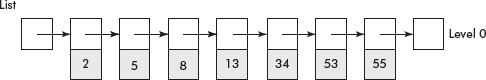
Fig. 10.24 A sorted linked list
It may be noted that the time complexity of various operations such as search, insertion, deletion, etc. on a sorted linked list is O(N).
Let us now add extra links in such a manner that every alternative node is skipped. The arrangement is shown in Figure 10.25. The chain of extra links is called level 1. The head node is said to have height equal to 1.
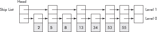
Fig. 10.25 A skip list with level 1
Now, we carry on to add another level of links, i.e., level 2 wherein every alternate node of level 1 is skipped as shown in Figure 10.26. The height of head node has become 2.
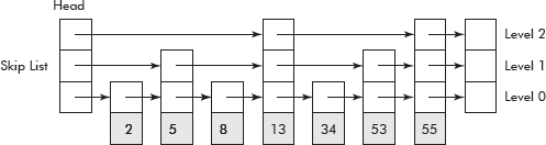
Fig. 10.26 A skip list with level2
The levels of links are added till we reach a stage where the link from head node has reached almost to the middle element of the linked list as has happened in Figure 10.26.
It may be noted that in level 1, links point to every second element in the list. In level 2, the links point to every fourth element in the list. Thus, it can be deduced that a link in the ith level will point to 2*ith element in the list. A point worth noting is that the last node of the skip list is pointed by links of all levels.
Now the search within the skip list shall take O(log n) time as it will follow binary search pattern. For example, the search for ‘53’ will follow the route shown in Figure 10.27.
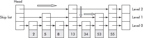
Fig. 10.27 The path followed for searching ‘53’ in the list
The algorithm that searches a value VAL in the skip list is given below:
Algorithm skipListSearch ()
  {
    curPtr = Head;
    For (I = N; I > 1; I−−)
    {
      while (DATA (curPtr[i] < VAL)
      CurPtr[I] = NEXT (CurPtr [I]);
      If (DATA (curPtr[I])) == VAL) ; return success;
    }
    return failure;
  }
It may be noted that insertion and deletion operations in the list will disturb the balance of the skip list and many levels of pointer adjustment would be required to redistribute the levels of pointers and heights of head and intermediate nodes.
10.4 B-TREES
A binary search tree (BST) is an extremely useful data structure as far as search operations on static data items is concerned. The reason is that static data can be so arranged that the BST generated out of the data is almost height balanced. However, for very large data stored in files, this data structure becomes unsuitable in terms of number of disk accesses required to read the data from the disk. The remedy is that each node of BST should store more than one record to accommodate the complete data of the file. Thus, the structure of BST needs to be modified. In fact, there is a need to extend the concept of BST so that huge amount of data for search operations could be easily handled.
We can look upon a BST as a two-way search tree in which each node (called root) has two subtrees—left subtree and right subtree, with following properties:
- The key values of the nodes of the left subtree are always less than the key value of the root node.
- The key values of the nodes of the right subtree are always more than the key value of the root node.
The concept of two-way search tree can be extended to create an m-way search tree having node structure shown in Figure 10.28.
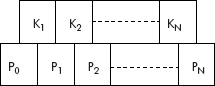
Fig. 10.28 M-way tree
The m-way tree has following properties:
- Each node has any number of children from 2 to M, i.e., all nodes have degree <= M, where M >= 2.
- Each node has keys (K1 to Kn) and pointers to its children (P0 to Pn), i.e., number of keys is one less than the number of pointers. The keys are ordered, i.e., Ki < Ki+1 for 1 <= i < n.
- The subtree pointed by a pointer Pi has key values less than the key value of Ki+1 for 1 <= i < n.
- The subtree pointed by a pointer Pn has key values greater than the key value of Kn.
- All subtrees pointed by pointers Pi are m-way trees.
It may be noted that all keys in the subtree to the left of a key are predecessors of the key and that on the right are successors of the key as shown in Figure 10.29. The m-way tree shown in the figure is of the order 3, i.e., m = 3.
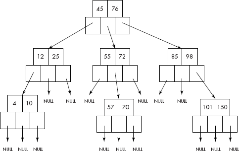
Fig. 10.29 An m-way search tree
A close look at the m-way tree suggests that it is a multilevel index structure. In order to have efficient search within an m-way tree, it should be height balanced. In fact, a height balanced m-way tree is called as B-tree. A precise definition of a B-tree is given below.
A B-tree of order m, has the following properties:
- The root has at least two children. If the tree contains only a root, i.e., it is a leaf node then it has no children.
- An interior node has between |m/2| and m children.
- Each leaf node must contain at least |m/2| – 1 children.
- All paths from the root to leaves have the same length, i.e., all leaves are at the same level making it height balanced.
Consider the B-tree given in Figure 10.30. It is of order 5 because all the internal nodes have at least |5/2| = 3 children and two keys. In fact, the maximum number of children and keys are 5 and 4, respectively. As per rule number 3, each leaf node must contain at least |5/2| − 1 = 2 keys.
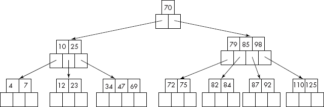
Fig. 10.30 A B-tree of size 5
It may be noted that the node of a B-tree, by its nature, can accommodate more than one key. We may design the size of a node to be as large as a block on the disk (say a sector). As a block is read at a time from the disk, compared to a normal BST, less number of disk accesses would be required to read/write data from the disk.
The following operations can be carried out on a B-tree:
- Searching a B-tree
- Inserting a new key in B-tree
- Deleting a key from a B-tree
10.4.1 Searching a Key in a B-Tree
A key K can be searched in a B-tree in a fashion similar to a BST. The search within a node, including root, follows the following algorithm:
Algorithm searchBTree()
  {
    Step
      1. Compare K with Ki for 1 <= i <= n.
      2. If Ki == K, then report search successful and return.
      3. Find the location i such that Ki <= K < K<i+1
      4. Move to the child node pointed by Pi.
      5. If Pi is equal to NULL, then report failure and return else repeat
         steps 1 to 4.
  }
The search for K = 82 will follow the path as shown in Figure 10.31.

10.4.2 Inserting a Key in a B-Tree
The insertion in a B-tree involves three primary steps: search – insert – (optional) split a node. The search operation finds the proper node wherein the key is to be inserted. The key is inserted in the node if it is already not full, else the node is split on the median (middle) key and the median number is inserted in the parent node. An algorithm that inserts a key in a B-tree is as follows:
Algorithm insertKey(Key)
  {
   Step
     1. Search the key in the B-tree.
     2. If it is found then prompt "Duplicate Key”.
     3. If not found, then mark the leaf. /* Unsuccessful search always
        ends at a leaf */
     4. If the leaf has empty location for the key, then insert it at the
        proper place.
     5. If the leaf is ’full’, then split the leaf into two halves at the
        median key.
     6. Move the median key from the leaf to its parent node and insert
        it there.
     7. Insert the key into the appropriate half.
     8. Adjust the pointers of the parent so that they point to the
        correct half.
     9. STOP
  }
Let us insert the following list of numbers into an empty B-tree:
3, 14, 7, 1, 8, 5, 11, 17, 13, 6, 23, 12, 20, 26
The trace of the above algorithm on the list of numbers is given in Figures 10.32 and 10.33.
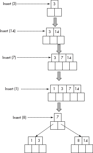
Fig. 10.32 Insertion of keys in a B-tree
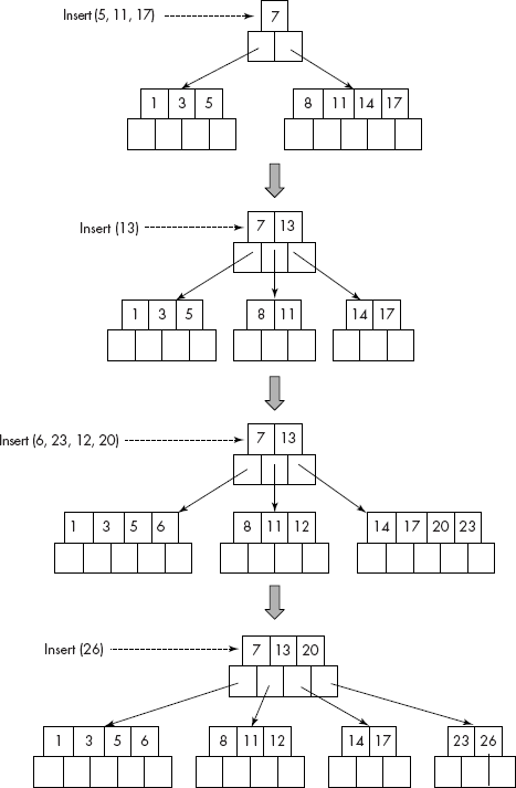
Fig. 10.33 Insertion of keys in a B-tree
10.4.3 Deleting a Key from a B-Tree
Deletion of a key from a node of B-tree has to be done with lot of care because it might violate the basic properties of the B-tree itself. For example, one must consider the following cases:
- After the deletion of a key in a leaf node, if the degree of the node decreases below the minimum degree of the tree then the siblings must be combined to increase the degree to the acceptable level.
Consider the deletion of K = 8 from the B-tree given in Figure 10.34.
Since the key (8) is in the leaf of the B-tree and its deletion does not violate the degree of that leaf, the key is deleted and the other elements in the node are appropriately shifted to maintain the order of the keys.
If the node is internal and has children, the children must be rearranged so that the basic properties of the B-tree are conformed to. In fact, we find its successor from the leaf node. If key is K and its successor is S, then S is deleted from the leaf node. Finally, S replaces the K.
Consider the deletion of 20 from the B-tree of Figure 10.35.
It may be noted that 23, the successor of 20, has been deleted from the child of node containing 20. The successor (23) has replaced the key (20) as the final step.
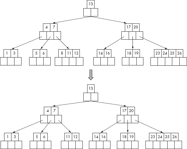
Fig. 10.34 Deletion of a key from a leaf of the B-tree
Fig. 10.35 Deletion of a key from an internal node of the B-tree
Consider the deletion of 19 from the B-tree of Figure 10.36.
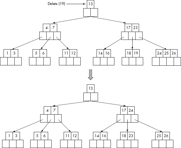
Fig. 10.36 Deletion of a key from a leaf causing violation
It may be noted that although the node containing 19 is a leaf node, the deletion violates the property that there should be at least two keys in the leaf node of a B-tree of order 5. Therefore, if an immediate sibling (left or right) has an extra key, then a key is borrowed from the parent (23) that is stored in place of the deleted key (19). The extra key (24) from the sibling is shifted to the parent as shown in Figure 10.36.
Let us finally consider the case of deletion of key (5). The deletion of 5 leaves no extra key in the leaf and its siblings (left or right) have also no extra keys to donate. Therefore, the parent key (4) is moved down and the siblings are combined as shown in Figure 10.37(a).
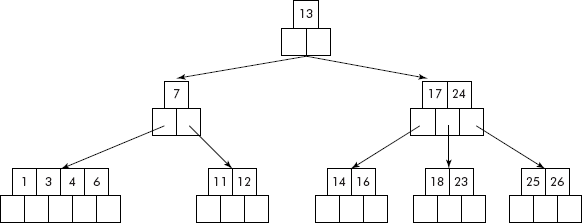
Fig. 10.37 (a) B-tree after deletion of key, k = 5
The moving down of 4 has caused a new problem that the parent node now contains only one key 7 (see Figure 10.37), which is another violation. As its sibling is also not having an extra key, the siblings need to be combined and bring 13 from the parent node. The final tree after adjustment is shown in Figure 10.37(b). However, the height of the tree has reduced by 1.
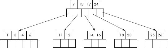
Fig. 10.37 (b) B-tree after double violation
Note: From the above discussion, it is clear that the insertion, and especially deletion, is a complicated operation in B-trees. Therefore, the size of leaf nodes is kept as large as 256 or more so that insertion and deletion do not demand rearrangement of nodes.
10.4.4 Advantages of B-trees
- As the size of a node of a B-tree is kept as large as 256 or more, the height of the tree becomes very small. Such a node supports children in the range of (128 to 256). Therefore, insertion and deletion operations will generally remain within the limit without causing over- or underflow of the node.
- As the height of a B-tree is very small, the key being searched is normally found at a shallow depth.
- If the root and next level of nodes are kept in the main memory (RAM), more than a million records of file can be indexed. Consequently, fewer disk accesses would be required to read the required record from the disk.
10.5 SEARCHING BY HASHING
In system programming, search is a very widely used operation. An assembler or a compiler very frequently searches the presence of a token in a table such as symbol table, opcode table, literal table etc. Earlier in the book, following techniques have been discussed for search operations:
- Linear search
- Binary search
- Binary search trees
Averagely, the linear search requires O(n) comparisons to search an element in a list. On the other hand, the binary search takes O(log n) comparisons to search an element in the list but it requires the list should already be sorted.
Some applications such as direct files, require the search to be of order O(1) in the best case i.e. the time of search should be independent of the location of the element or key in the storage area. In fact, in this situation a hash function is used to obtain a unique address for a given key or a token. The term ‘hashing’ means key transformation. The address for a key is derived by applying an arithmetic function called ‘hash’ function on the key itself. The address so generated is used to store the record of the key as shown in Fig. 10.38.
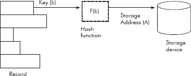
Fig. 10.38 Direct address generation
In the following section, various hashing functions are discussed.
10.5.1 Types of Hashing Functions
Many hashing functions are available in the literature. Most of the efficient hash functions are complex. For instance, MD5 and SHA-1 are complex but very efficient hash functions used for cryptographic applications. However, for searching records or tokens in files or tables, even simple hash functions give good results. Some of the common Hashing functions are described below.
- Midsquare method: The value of the key K is squared and afterwards a suitable number of digits from the middle of K2 is chosen to be the address of the record on the disk. Let us assume that 4th and 5th digit from the right of K2 will be selected as the hash address as shown below :
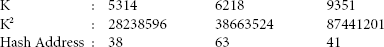
It may be noted that the records with K = 5314, 6218, and 9351, would be stored at addresses 38, 63, and 41 respectively.
- Division method: In this method the key K is divided by a prime number where a prime number is a number that is evenly divisible (without a remainder) only by one or by the number itself. After the division, the quotient is discarded and the remainder is taken as the address. Let us consider the examples given below
(i) Let key K = 189235 Prime number (p) = 41 (say) → Hash address = K mod p = 189235 mod 41 = 20 ( remainder ) (ii) Let key K = 5314 Prime number (p) = 41 → Hash address = K mod p = 5314 mod 41 = 25 ( remainder ) - Folding method: In this method, the key is split into pieces and a suitable arithmetic operation is done on the pieces. The operations can be add, subtract, divide etc. Let us consider the following examples:
- Let key K = 189235
Let us split it into two parts 189 and 235
By adding the two parts we get,
189
235
Hash address 424
- Let key K = 123529164
Splitting the key into pieces and adding them, we get
Let us split it into three parts 123, 529 and 164
By adding the two parts we get,
123
529
164
Hash address 816
- Let key K = 189235
It may be observed from the examples given above, that there are chances that the records with different key values may hash to the same address. For example, in folding technique, the keys 123529164 and 529164123 will generate the same address, i.e., 816. Such mapping of keys to the same address is known as a collision and the keys are called as synonyms.
Now, to manage the collisions, the overflowed keys must be stored in some other storage space called overflow area. The procedure is described below:
- When a record is to be stored, a suitable hashing function is applied on the key of the record and an address is generated. The storage area is accessed, and, if it is unused, the record is stored there. If there is already a record stored, the new record is written in the overflow area.
- When the record is to be retrieved, the same process is repeated. The record is checked at the generated address. If it is not the desired one, the system looks for the record in the overflow area and retrieves the record from there.
Thus, synonyms cause loss of time in searching records, as they are not at the expected address. It is therefore essential to devise hash algorithms which generate minimum number of collisions. The important features required in a hash algorithm are given in the following section.
10.5.2 Requirements for Hashing Algorithms
The important features required in a Hash algorithm or functions are :
- Repeatable: A capability to generate a unique address where a record can be stored and retrieved afterwards.
- Even distribution: The records of a file should be evenly distributed throughout the allocated storage space.
- Minimum collisions: It should generate unique addresses for different keys so that number of collisions can be minimized.
Nevertheless, the collisions can be managed by using suitable methods as discussed in next section:
10.5.3 Overflow Management (Collision handling)
The following overflow management methods can be used to manage the collisions.
- Chaining: The overflowed records are stored in a chain of collisions maintained as linked lists as shown in Figure 10.39
Assuming that (K mod 10) was taken as the hash function. Therefore, the keys with values 0, 10, 20, 30 etc. will map on the same address i.e. 0 and their associated records are stored in a linked list of nodes as shown in figure. Similarly 19, 9, and 59 will also map on the same address i.e. 9 and their associated records stored in a linked list of nodes.
It may be noted that when a key K is searched in the above arrangement and if it is not found in the head node then it is searched in the attached linked list. Since the linked list is a pure sequential data structure, the search becomes sequential. A poor hash function will generate many collisions leading to creation of long linked lists. Consequently the search will become very slow. The remedy to above drawback of chaining is rehashing.
- Rehashing: When the address generated by a hash function F1 for a key Kj collides with another key Ki then another hash function F2 is applied on the address to obtain a new address A2. The collided Key Kj is then stored at the new address A2 as shown in Fig. 10. 40
It may be noted that if the space referred to by A2 is also occupied, then the process of rehashing is again repeated. In fact rehashing is repeatedly applied on the intermediate address until a free location is found where the record could be stored.
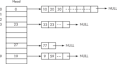
Fig. 10.39 Chaining
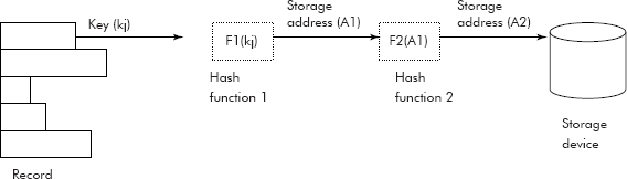
Fig. 10.40 Rehashing
EXERCISES
- When does a binary search tree (BST) become a skewed tree?
- What is an AVL Tree? What are its advantages over a BST?
- Write an explanatory note on AVL rotations.
- For the AVL Tree shown in Figure 10.41, label each node in the AVL Tree with the correct balance factor. Use 1 for left higher, 0 for equal height, and −1 for right higher subtrees.
- For the AVL Tree shown in Fig. 10.41, draw the final AVL Tree that would result from performing the actions indicated from (a) to (e) listed below:
- Insert the key 10.
- Insert the key 95.
- Insert the key 80, and then insert the key 77.
- Insert the key 80, and then insert the key 83.
- Insert the key 45.
Note: Always start with the given tree, the questions are not accumulative. Also, show both the data value and balance factor for each node.
- Define set data structure. How are they different from arrays? Give examples to show the applications of the set data structures.
- Write an algorithm that computes the height of a tree.
- Write an algorithm that searches a key K in an AVL Tree.
- What are the various cases of insertion of a key K in an AVL Tree?
- Define the terms: null set, subset, disjoint set, cardinality of a set, and partition.
- What are the various methods of representing sets?
- Write an algorithm that takes two sets S1 and S2 and produces a third set S3 such that S3 = S1 ⋃ S2.
- Write an algorithm that takes two sets S1 and S2 and produces a third set S3 such that S3 = S1 ∩ S2.
- Write an algorithm that takes two sets S1 and S2 and produces a third set S3 such that S3 = S1 − S2.
- How are web pages managed by a search engine?
- Give the steps used for colouring a black and white photograph.
- Write a short note on spell checker as an application of sets.
- You are given a set of persons P and their friendship relation R, that is, (a, b) Є R if a is a friend of b. You must find a way to introduce person x to person y through a chain of friends. Model this problem with a graph and describe a strategy to solve the problem.
- The subset-sum problem is defined as follows:
Input: a set of numbers A = {a1, a2, … , aN} and a number x;
Output: 1 if there is a subset of numbers in A that add up to x.
Write down the algorithm to solve the subset-sum problem.
- What is a skip list? What is the necessity of adding extra links?
- Write an algorithm that searches a key K in a skip list.
- What is an m-way tree.
- Define a B-tree. What are its properties?
- Write an algorithm for searching a key K, in a B-tree.
- Write an algorithm for inserting a key K, in a B-tree.
- Write an explanatory note on deletion operation in a B-tree.
- What are the advantages of a B-tree.
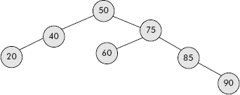
Fig. 10.41 An AVL tree