
Chapter 2
Data Structures and Algorithms: An Introduction
CHAPTER OUTLINE
2.1 OVERVIEW
A normal desktop computer is based on Von Neumann architecture. It is also called a stored program computer because the program’s instructions and its associated data are stored in the same memory as shown in Figure 2.1.
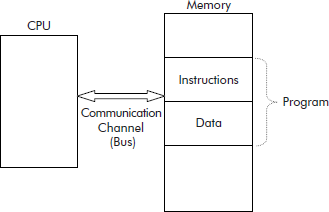
Fig. 2.1 The stored program computer
The program instructions tell the system what operation is to be performed and on what data.
The above model is based on the fact that every practical problem that needs to be solved must have some associated data. Let us consider a situation where a list of numbers is to be sorted in ascending order. This problem obviously has the following two parts:
- The list: say 9, 8, 1, −1, 4, 2, 6, 15, 3
- A procedure to sort the given list of numbers.
It may be noted that elements of list and the procedure represent the data and program of the problem, respectively.
Now, the efficiency of the program would primarily depend upon the organization of data. When the data is poorly organized, then the program cannot efficiently access it. For instance, the time taken to open the lock of your house depends upon where you have kept the key to it: in your hand, in front pocket, in the ticket pocket of your pant or the inner pocket of your briefcase, etc. There may be a variety of motives for selecting one or the other of these places to keep the key. Key in the hand or in the front pocket would be quickly accessible as compared to other places whereas the key placed in the inner pocket of briefcase is comparatively much secured. For similar reasons, it is also necessary to choose a suitable representation or structure for data so that a program can efficiently access it.
2.2 CONCEPT OF DATA STRUCTURES
In fact the data, belonging to a problem, must be organized for the following basic reasons:
- Suitable representation: Data should be stored in such a manner that it represents the various components of the problem.
For example, the list of numbers can be stored in physical continuous locations. Arrays in ‘C’ can be used for the required representation as shown in Figure 2.2.
- Ease of retrieval: The data should be stored in such a manner that the program can easily access it.
As an array is an index–value pair, a data item stored in the array (see Figure 2.2) can be very easily accessed through its index. For example, List [5] will provide the data item stored at 5th location, i.e. ‘2’. From this point of view, the array is a random-access structure.
- Operations allowed: The operations needed to be performed on the data must be allowed by the representation.
For example, component by component operations can be done on the data items stored in the array. Consider the data stored in List of Figure 2.2. For the purpose of sorting, the smallest number must come to the head of the list. This shall require the following two operations:
- Visit every element (component) in the list to search the smallest and its position (’−1’ at location 3).
- Exchange the smallest with the number stored at the head of the list (exchange ‘−1’stored at location 3 with ‘9’ stored at location 0). This can be easily done by using a temporary location (say Temp) as shown below:
              Temp    = List[0];
              List[0] = List[3];
              List[3] = Temp;
Fig. 2.2 List stored in physical continuous locations
The new contents of the List are as shown in Figure 2.3.
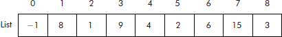
Fig. 2.3 Contents of the List after exchange operation
The operations 1 and 2, given above, can be repeated on the unsorted part of the List to obtain the required sorted List.
From above discussions, it can be concluded that an array provides a suitable representation for the storage of a list of numbers. Such a representation is also called a data structure. Data structure is a logical organization of a set of data items that collectively describe an object. It can be manipulated by a program. For example, array is a suitable data structure for a list of data items.
It may be observed that if the array called ‘List’ represents the data structure then the operations carried out in steps 1 and 2 define the algorithm needed to solve the problem. The overall performance of a program depends upon the following two factors:
- Choice of right data structures for the given problem.
- Design of a suitable algorithm to work upon the chosen data structures.
2.2.1 Choice of Right Data Structures
An important step of problem solving is to select the data structure wherein the data will be stored. The program or algorithm would then work on this data structure and give the results.
A data structure can either be selected from the built-in data structures offered by the language or by designing a new one. Built-in data structures in ‘C’ are arrays, structures, unions, files, pointers, etc.
Let us consider a situation where it is required to create a merit list of 60 students. These students appeared in a class examination. The data of a student consists of his name, roll number, marks, percentage, and grade. Out of many possibilities, the following two choices of data structures are worth considering:
Choice I: The various data items related to a student are: name, roll number, marks, percentage, and grade. The total number of students is 60. Therefore, the simplest choice would be to have as many parallel lists as there are data items to be represented. The arrangement is shown Figure 2.4.
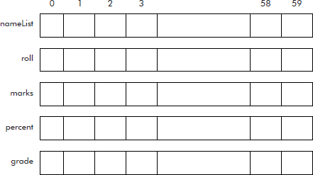
Fig. 2.4 Parallel lists for student data
An equivalent declaration for data structure of Figure 2.4 is given below:
  char  nameList[60][15];
  int   roll[60];
  int   marks[60];
  float percent[60];
  char  grade[60];
Now in the above declaration, every list has to be considered as individual. The generation of merit list would require the list to be sorted. The sorting process would involve a large number of exchange operations. For each list, separate exchange operations would have to be written. For example, the exchange between data of ith and jth student would require the following operations:
    char tempName[15],chTemp;
    int i,j, temp;
    float fTemp;

    strcpy (tempName, nameList[i]);
    strcpy (nameList[i], nameList[j]);
    strcpy (nameList[j], tempName);

    temp = roll[i];
    roll[i] = roll[j];
    roll[j] = temp;

    temp = marks[i];
    marks[i] = marks[j];
    marks[j] = temp;

    fTemp = percent[i];
    percent[i] = percent[j];
    percent[j] = fTemp;

    chTemp = grade[i];
    grade[i] = grade[j];
    grade[j] = chTemp;
Though the above code may work, but it is not only a clumsy way of representing the data but would require a lot of typing effort also. In fact, as many as fifteen statements are required to exchange the data of ith student with that of jth student.
Choice II: From the built-in data structures, the struct can be selected to represent the data of a student as shown below:
    struct student {
     char  name[15];
     int   roll;
     int   marks;
     float  percent;
     char  grade;
     };
Similarly, from built-in data structures, an array called studList can be selected to represent a list. However, in this case each location has to be of type student which itself is a structure. The required declaration is given below:
struct student studList [60];
It may be noted that the above given array of structures is a user-defined data structure constructed from two built-in data structures: struct and array. Now in this case, exchange between data of ith and jth student would require the following operations:
     int i,j;
     struct student temp;
     temp = studList[i];
     studList [i] = studList [j];
     studList [j] = temp;
Thus, only three statements are required to exchange the data of ith student with that of jth student.
A comparison of the two choices discussed above establishes that Choice II is definitely better than Choice I as far as the selection of data structures for the given problem is concerned. The number of lines of code of Choice II is definitely less than the Choice I. Moreover, the code of Choice II is comparatively easy and elegant.
From the above discussion, it can be concluded that choice of right data structures is of paramount importance from the point of view of representing the data belonging to a problem.
2.2.2 Types of Data Structures
A large number of data structure are available to programmers that can be usefully employed in a program. The data structures can be broadly classified into two categories: linear and non-linear.
- Linear data structures: These data structures represent a sequence of items. The elements follow a linear ordering. For instance, one-dimensional arrays and linked lists are linear data structures. These can be used to model objects like queues, stacks, chains (linked lists), etc., as shown in Figure 2.5.
A linear data structure has following two properties:
- Each element is ‘followed by’ at most one other element.
- No two elements are ‘followed by’ the same element.
For example, in the list of Figure 2.3, the 2nd element (’1’) is followed by 3rd element (’9’) and so on.
- Non-linear data structures: These data structures represent objects which are not in sequence but are distributed in a plane. For instance, two-dimensional arrays, graphs, trees, etc. are non-linear data structures. These can be used to model objects like tables, networks and hierarchy, as shown in Figure 2.6.
The tree structure does not follow the first property of linear data structures and the graph does not follow any property of the linear data structures. A detailed discussion on this issue is given later in the book.
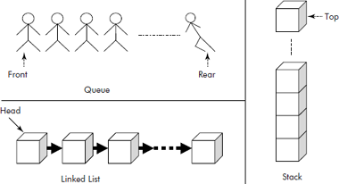
Fig. 2.5 Linear data structures
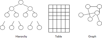
Fig. 2.6 Non-linear data structures
2.2.3 Basic Terminology Related with Data Structures
The basic terms connected with the data structures are:
- Data element: It is the most fundamental level of data. For example, a Date is made up of three parts: Day, Month, and Year as shown in Figure 2.7. The Date is called a data object and DD, MM, and YY are called the data elements or data items.
It may be noted that the data object denotes a group and the data elements denote atomic entities.
- Primitive data types: It is type of data that a variable may hold. For example, int, float, char, etc. are data types.
- Data object: It is a set of elements. For example, the set of fruit ‘F’ refers to the set F = {’mango’, ‘orange’, ‘grapes’….}. Similarly, a set of counting numbers ‘C’ refers to the set C = {1, 2, 3, 4….}.
- Data structure: It is a set of related elements. A set of operations that are allowed on the elements of the data structure is defined.
- Constant: It is the memory location that does not change its contents during the execution of a program.
- Variable: It is the most fundamental aspect of any computer language and can be defined as a location in the memory wherein a value can be manipulated, i.e., stored, accessed, and modified.
Fig. 2.7 Data elements of data object Date
2.3 DESIGN OF A SUITABLE ALGORITHM
After selecting the data structures, an algorithm, based on the data structure, needs to be designed. The set of rules that define how a particular problem can be solved in a finite sequence of steps is called an algorithm. An algorithm written in a computer language is called a program. An algorithm can be defined as a finite sequence of instructions, each of which has a clear meaning and can be executed with a finite amount of effort in finite time.
A computer is simply a machine with no intelligence. In fact, the processor of the computer is a passive device that can only execute instructions. Therefore, the computer must be instructed in unambiguous steps such that it follows them one after the other to perform the given task. Thus, it becomes programmer’s duty to precisely define his problem in the form of an algorithm, i.e., unambiguous steps written in simple English. The desirable features of an algorithm are:
- Each step of the algorithm should be simple.
- It should be unambiguous in the sense that the logic should be crisp and clear.
- It should be effective, i.e., it must lead to a unique solution of the problem.
- It must end in a finite number of steps.
- It should be as efficient as possible.
Accordingly, an algorithm has the following characteristics:
- Input: This part of the algorithm reads the data of the given problem.
- Process: This part of the algorithm does the required computations in simple steps.
- Finiteness: The algorithm must come to an end after a finite number of steps.
- Effectiveness: Every step of the algorithm must be accurate and precise. It should also be executable within a definite period of time on the target machine.
- Output: It must produce the desired output.
Thus, we can say that the algorithm tells the computer when to read data, compute on it, and write the answers.
2.3.1 How to Develop an Algorithm?
In order to develop an algorithm, the problem has to be properly analysed. The programmer has to understand the problem and come out with a method or logic that can solve the problem. The logic must be simple and adaptable on a computer. The following steps can be suggested for developing an algorithm:
- Understand the problem.
- Identify the output of the problem.
- Identify inputs required by the problem and choose the associated data structures.
- Design a logic that will produce the desired output from the given inputs.
- Test the algorithm for different sets of input data.
- Repeat steps 1 to 5 till the algorithm produces the desired results for all types of input and rules.
While solving problems with the help of computers, the following facts should be kept in mind:
"A location in the main memory has the property: Writing-in is destructive and Reading-out is non-destructive”. In simple words, we can say that if a value is assigned to a memory location, then its dprevious contents will be lost. However, if we use the value of a memory location then the contents of the memory do not change, i.e., it remains intact. For example, in the following statement, the value of variables B and C are being used and their sum is stored in variable A
A = B + C
where, the symbol ‘=’ is an assignment operator.
If previous values of A, B, C were 15, 45, 20, respectively then after execution of the above statement, the new contents of A, B, C would be 65, 45, and 20, respectively.
Consider the following statement:
Total = Total + 100;
The abnormal looking statement is very much normal as far as computer memory is concerned. The statement reveals the following fact:
"Old value of variable ‘Total’ is being added to an integer 100 and the result is being stored as new value in the variable ‘Total’, i.e., replacing its old contents with the new contents.”
After the execution of the statement with old contents of ‘Total’ (say 24), the new contents of ‘Total’ will be 124.
2.3.1.1 Identifying Inputs and Outputs
It is very important to identify inputs and outputs of an algorithm. The inputs to an algorithm mean the data to be provided to the target program through input devices such as keyboard, mouse, input file, etc. The output of the algorithm means the final data to be generated for the output devices such as monitor, printer, output file, etc.
The inputs and outputs have to be identified at the beginning of the program development. The most important decision is to differentiate between major and minor inputs and outputs. The minor inputs are sometimes omitted at the algorithm development stage. The other important issue is to find at which part of the program the inputs would be required and the output generated.
Example 1: Let us reconsider the problem of sorting a given list of numbers. In this case, the required inputs are:
- List of numbers
- Size of list
- Type of numbers to be stored in the list
- In which order to be sorted
The outputs are:
- The sorted list
- Message for asking the size of the list
- Message for displaying the output list
The messages are the minor outputs.
After identifying the inputs and the outputs, the additional information must be specified before writing the final algorithm.
Input specifications
- In what order and format, the input values will be read?
- What are the lower and upper limits of the input values? For example, the size of the list should not be less than zero and its type has to be necessarily an integer.
- When to know that there is no more input to be read, i.e., what marks the end of the list?
- In what order and format the outputs values will be produced?
- What types of values to be produced with what spacing i.e., decimal spacing, significant digits, etc.
- What main headings and column headings to be printed on the output page.
2.3.2 Stepwise Refinement
We know that if there is even a small logical error in a program, the compiler cannot detect it. The year 2000 problem (Y2K problem) is a glaring example of this type. Thus, an algorithm requires a very careful design, especially pertaining to a large and complex problem.
In order to design an algorithm, the programmer must adopt some methodological approach such as modular/stepwise refinement approach of structured programming techniques. Stepwise refinement uses the “divide and conquer” strategy. In this technique, the problem is divided into a number of steps. Each step is described by a sub-problem which is smaller and simpler as compared to the original program. The sub-problem is again divided into still smaller steps and so on. The refinement continues till we reach to a stage where the steps become fairly simple to implement.
Example 2: Suppose the following table is to be printed on the screen.
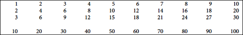
The problem at hand is “How to print the table”. The first version of the algorithm is given below:
  Algorithm Print_Table Ver1.
 {
   Step 1. Print table
 }
When we look at the table, we find that the table is nothing but a collection of rows and we have to print only 10 rows. So, the problem has been reduced to printing a row 10 times. The second refined version of the algorithm is given below:
  Algorithm Print_Table Ver2.
 {
   Step
    1. Row = 1
    2. Print the row
    3. Row = Row + 1
    4. If Row <= 10 repeat steps 2 and 3
    5. Stop
 }
Now our focus is on “how to print a row”. A closer look at the problem suggests that a row is nothing but a collection of columns and we have to print only 10 columns for each row. The third refined version of the algorithm is given below:
 Algorithm Print_Table Ver3.
 {
   Step
    1. Row = 1
    2. Col = 1
       2.1 Print the col.
       2.2 Col = Col + 1
       2.3 If Col <= 10 repeat steps 1 and 2
       2.4 Go to a new line.
    3. Row = Row + 1
    4. If Row <=10 repeat steps 2 and 3
    5. Stop.
 }
Now our concern is “how to print a column”. We find that it is very simple, i.e., we get the value to be printed by multiplying the values contained in the variables Row and Col. The final version of the refined algorithm is given below:
 Algorithm Print_Table Ver3.
 {
   Step
    1. Row = 1
    2. Col = 1
       2.1 ColVal = Row * Col
       2.2 Print the ColVal.
       2.3 Col = Col + 1
       2.4 If Col <= 10 repeat steps 1 and 3
       2.5 Go to a new line.
    3. Row = Row + 1
    4. If Row <=10 repeat steps 2 and 3
    5. Stop.
 }
The programmer stops at this stage where he finds that the step(s) is trivial and can be easily implemented.
2.3.3 Using Control Structures
Every language supports sequence control structures. These structures can be easily used towards writing a program for a given problem.
(1) Sequence structure: The order in which the statements or statement blocks are written within a pair of curly braces ({,}) in an algorithm are sequentially executed by the computer.
Example 3: Write an algorithm that computes the area of a triangle.
Solution: The solution is trivial. The inputs are base and height. The following formula will be used for the computation of the area of triangle:
Area = ½ * base * height
where area is the output to be displayed. The simple sequence structure required for this problem is given below:
 Algorithm AreaTriangle ()
 {
   Step
    1. Read base, height;
    2. Area = 0.5 * base * height;
    3. Print Area;
    4. Stop
 }
It may be noted that in a sequence structure:
- The statements are executed sequentially.
- The statements are executed one at a time.
- Each statement is executed only once.
- No statement is repeated.
- The execution of the last statement marks the end of the sequential structure.
(2) Selection (conditional control) structure: The selection or decision structure is used to decide whether a statement or a block is to be executed or not. The decision is made by testing whether a condition is true or false. The if-else ladder structure can be used for this purpose.
Example 4: Write an algorithm that prints the biggest of given three unique numbers.
Solution:
Input: Three numbers: Num1, Num2, and Num3
Type of numbers: integer.
Output: Display the biggest number and a message in this regard.
 Algorithm Biggest ()
 {
    Step
     1. Read Num1, Num2, Num3;
     2. If (Num1 > Num2)
        2.1 If (Num1 > Num3)
            Print "Num1 is the largest"
            Else
            Print "Num3 is the largest"
        Else
        2.2 If (Num2 > Num3)
            Print "Num2 is the largest"
            Else
            Print "Num3 is the largest"
     3. Stop
 }
(3) Iteration: The iteration structure is used to repeatedly execute a statement or a block of statements. The loop is repeatedly executed until a certain specified condition is satisfied.
Example 5: Write an algorithm that finds the largest number from a given list of numbers.
Solution:
Input: List of numbers, size of list, prompt for input.
Type of numbers: integer.
Output: Display the largest number and a message in this regard.
The most basic solution to this problem is that if there is only one number in the list then the number is the largest. Therefore, the first number of the list would be taken as largest. The largest would then be compared with the rest of the numbers in the list. If a number is found larger than the current largest, then it is stored in the largest. This process is repeated till the end of the list. For iteration, For loop can be employed.
The concerned algorithm is given below:
  Algorithm Largest
  {
    Step
     1. Prompt "Enter the size of the list”;
     2. Read N;
     3. Prompt "Enter a Number”;
     4. Read Num;
     5. Largest = Num;     /* The first number is the largest*/
     6. For (I = 2 to N)
        {
          6.1 Prompt "Enter a Number"
          6.2 Read Num
          6.3 If (Num > Largest) Largest = Num
        }
     7. Prompt "The largest Number =”
     8. Print Largest;
     9. Stop
  }
It may be noted here that if a loop terminates after a number of iterations, then the loop is called a finite loop. On the other hand if a loop does not terminate at all and keeps on executing endlessly, then it is called an infinite loop.
(4) Use of accumulators and counters: Accumulator is a variable that is generally used to compute sum or product of a series. For example, the sum of the following list of numbers can be computed by initializing a variable (say ‘Total’) to zero.
The 1st number of the list is added to Total and then the 2nd, 3rd and so on till the end of the list. Finally, the variable Total would get the accumulated sum of the list given above.
Example 6: Write an algorithm that reads a list of 50 integer values and prints the total of the list.
Solution: Let us assume that a variable called ‘sum’ would be used as an accumulator. A variable called Num would be used to read a number from the input list one at time. For loop will be employed to do the iteration.
  Algorithm SumList
  {
   Step
    1. Sum =0;
    2. For (I = 1 to 50)
       {
        2.1 Read Num;
        2.2 Sum = Sum + Num; /* The accumulation of the list */
       }
    3. Prompt "The sum of the list =”;
    4. Print Sum;
    5. Stop
  }
It may be noted that for product of a series, the accumulator is initialized to 1.
Counter is a variable used to count number of operations/actions performed in a loop. It may also be used to count number of members present in a list or a set of items.
The counter variable is generally initialized by 0. On the occurrence of an event/operation, the variable is incremented by 1. At the end of the counting process, the variable contains the required count.
Example 7: Write an algorithm that finds the number of zeros present in a given list of N numbers.
Solution: A counter variable called Num_of_Zeros would be used to count the number of zeros present in a given list of numbers. A variable called Num would be used to read a number from the input list one at time. For loop will be employed to do the iteration.
The Algorithm is given below:
  Algorithm Count_zeros()
  {
    Step
     1. Num_of_zeros = 0;
     2. For (I = 1 to N)
        {
          2.1 Read Num;
          2.2 If (Num == 0)
              Num_of_zeros = Num_of_zeros +1;
        }
     3. Prompt "The number of zero elements =”;
     4. Print Num_of_zeros;
     5. Stop
  }
Example 8: Write a program that computes the sum of first N multiples of an integer called ‘K’, i.e.
sumSeries = 1*K + 2*K + 3*K + .........N*K
Solution: An accumulator called sumSeries would be used to compute the required sum of the series. As the number of steps are known (i.e., N), ‘For loop’ is the most appropriate for the required computation. The index of the loop will act as the counter.
Output: sumSeries
The program is given below:
  /* This program computes the sum of a series */
   #include <stdio.h>
   void main()
   {
      int sumSeries, i;
      int N; /* Number of terms */
      int K; /* The integer multiple*/
           printf(“
 Enter Number of terms and Integer Multiple”);
           scanf (“%d %d”, &N,&K);
           sumSeries = 0; /*Accumulator initialized */
           For (i=1; i<=N; i++)
           {
            sumSeries = sumSeries + i*K;
           }
          printf (“
 The sum of first %d terms = %d”, N, sumSeries);
 }
In fact, it can be concluded that irrespective of the programming paradigms, a general algorithm is designed based on following constructs:
- Sequence structure: Statement after statements are written in sequence in a program.
- Selection: Based on a decision (i.e., if-else), a section of statements is executed.
- Iteration: A group of statements is executed within a loop.
- Function call: At a certain point in program, the statement may call a function to perform a particular task.
It is the responsibility of the programmer to use the right construct at right place in the algorithm so that an efficient program is produced. A discussion on analysis of algorithms is given in next section.
2.4 ALGORITHM ANALYSIS
A critical look at the above discussion indicates that the data structures and algorithms are related to each other and have to be studied together. For a given problem, an algorithm is developed to solve it but the algorithm needs to operate on data. Unless the data is stored in a suitable data structure, the design of algorithm remains incomplete. So, both the data structures and algorithm are important for program development.
In fact, an algorithm requires following two resources:
- Memory space: Space occupied by program code and the associated data structures.
- CPU time: Time spent by the algorithm to solve the problem.
Therefore, an algorithm can be analyzed on two accounts: space and time. We need to develop an algorithm that efficiently makes use of these resources. But then, there are many ways to attack a problem and hence many algorithms at hand to choose from. Obviously, having decided the data structures, execution time can be a major criterion for selection of an algorithm.
As a first step, it is understandable that an algorithm would be fast for a small input data. For example, the search for an item in a list of 10 elements would definitely be faster as compared to searching the same item within a list of 1,000 elements. Therefore, the execution time T of an algorithm has to be dependent upon N, the size of input data. Now the question is how to measure the execution time T. Can we exactly compute the execution time? Perhaps not because there are many factors that govern the actual execution of program in a computer system. Some of the important factors are listed below:
- The speed of the computer system
- The structure of the program
- Quality of the compiler that has compiled the program
- The current load on the computer system.
Thus, it is better that we compare the algorithms based on their relative time instead of actual execution time.
The amount of time taken for completion of an algorithm is called time complexity of the algorithm. It is a theoretical estimate that measures the growth rate of the algorithm T(n) for large number of n, the input size. The time complexity is measured in terms of Big-Oh notation. A brief discussion on this notation is given in next section.
2.4.1 Big-Oh Notation
The Big-Oh notation defines that for a large number of input ‘n’, the growth rate of an algorithm T(n) is of the order of a function ‘g’ of ‘n’ as indicated by the following relation:
T(n) = O(g(n)).
The term ‘of the order’ means that T(n) is less than a constant multiple of g(n) for n >= n0. Therefore, for a constant ‘c’, the relation can be defined as given below:
T(n) <= c*g(n) where c >0.
From above relation, we can say that for a large value of n, the function ‘g’ provides an upper bound on the growth rate ‘T’.
Let us now consider the various constructs used by a programmer to write an algorithm.
(1) Simple statement: Let us assume that a statement takes a unit time to execute, i.e., 1. Thus, T(n) = 1 for a simple statement. To satisfy the Big-Oh condition, the above relation can be rewritten as shown below:
T(n) <= 1*1 where c = 1 and n0 = 0.
Comparing the above relation with relation 2.1, we get g(n) = 1. Therefore, the above relation can be expressed as:
T(n) = O(1)
(2) Sequence structure: The execution time of sequence structure is equal to the sum of execution time of individual statements present within the sequence structure.
Consider the following algorithm. It consists of a sequence of statements 1 to 4:
  Algorithm AreaTriangle
 {
   Step
    1. Read base, height;
    2. Area = 0.5 * base * height;
    3. Print Area;
    4. Stop
 }
The above algorithm takes four steps to complete.
Thus, T(n) = 4.
To satisfy the relation 2.1, the above relation can be rewritten as:
T(n) <= 4*1 where c = 4 and n0 = 0.
Comparing the above relation with relation 2.1, we get g(n) =1. Therefore, the above relation can be expressed as:
T(n) = O(1)
We can say that the time complexity of above algorithm is O(1), i.e., of the order 1.
(3) The loop structure: The loop structure iteratively executes statements written within its bound. If a loop executes for N iterations, it contains only simple statements.
Consider the algorithm Count_zeros of Example 7 which contains a loop. This algorithm takes the following steps for its completion
| No. of simple steps | = 4 (Steps 1, 3, 4, 5) |
| No. of Loops of steps 1 to N | = 1 |
| No. of statements within the loop | = 3 (1 comparison, 1 addition, 1 assignment) |
Thus, T(n) = 3*N + 4
Now for N >= 4, we can say that
3*N + 4 <= 3*N + N <= 4N
Therefore, we can say that
T(n) <= 4N where c = 4, n0 >= 4
T(n) = O(N)
Hence, the given algorithm has time complexity of the order of N, i.e., O(N). This indicates that the term 4 has negligible contribution in the expression: 3*N + 4.
Note: In case of nested loops, the time complexity depends upon the counters of both outer and inner loops. Consider the nested loops given below. This program segment contains ‘S’, a sequence of statements within nested loops I and J.
  For (I = 1; I <= N; I++)
  {
    For (J = 1; J <= N; J++)
    {
      S;
    }
  }
It may be noted that for each iteration of I loop, the J loop executes N times. Therefore, for N iterations of I loop, the J loop would execute N*N = N2 times. Accordingly, the statement S would also execute N2 times.
Thus, T(n) = N2
To satisfy the relation 2.1, the above relation can be rewritten as shown below:
T(n) <= 1 * N2 where c = 1 and n0 = 0.
Comparing the above relation with relation 2.1, we get g(n) = N2. Therefore, the above relation can be expressed as:
T(n) = O(N2)
Hence, the given nested loop has time complexity of the order of N2, i.e., O(N2).
Example 9: Compute the time complexity of the following nested loop:
   For (I = 1; I <= N; I++)
   {
     For (J = 1; J <= I; J++)
     {
       S;
     }
   }
Solution: In this nested loop structure, for an iteration of I loop, the J loop executes in an increasing order from 1 to N as given below:
1 + 2 + 3 + 4 +……. (N – 1) + N = N*(N + 1)/2 = N2/2 + N/2.
Thus, T(n) = N2/2 + N/2.
Now for N2 >= N/2, we can say that:
N2/2 + N/2 <= N2/2 + N2 <= 3 N2/2.
Therefore, we can say that
T(n) <= 3 N2/2 where, c = 3/2, n0 = N2
T(n) = O(N2)
Hence, the given algorithm has time complexity of the order of N2, i.e., O(N2). This indicates that the term N/2 has negligible contribution in the expression N2/2 + N/2.
(4) If-then-else structure: In the if-then-else structure, the then and else parts are considered separately. Consider the if-then-else structure given in Figure 2.8.
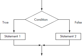
Fig. 2.8 The if-then-else structure
Let us assume that the ‘statement 1’ of then part has the time complexity T1 and that ‘statement 2’ of else part has the time complexity T2. The time complexity of if-then-else structure is taken to be the maximum of the two, i.e., max(T1, T2).
Example 10: Consider the following algorithm. Compute its time complexity.
   If (x > y)
     {
        x = x+1;
     }
    Else
     {
        For (i=1; i <= N, i++)
        {
          x = x+i;
        }
     }
Solution: It may be noted that in the above algorithm, the time complexity of ‘then’ and ‘else’ part are O(1) and O(N), respectively. The maximum of the two is O(N). Therefore, the time complexity of the above algorithm is O(N).
Example 11: compute the time complexity of the following relations:
- T(n) = 2527
- T(n) = 8*n + 17
- T(n) = 15*N2 + 6
- T(n) = 5*N3 + N2 + 2*N
Solution:
- T(n) = 2527 <= 2527*1, where c = 2527 and n0 = 0.
= O(1)
Ans. The time complexity = O(1)
- T(n) = 8*n + 17 <= 8*n + n <= 9 *n for c = 9 and n0 = 17
= O(N)
Ans. The time complexity = O(N)
- T(n) = 15*N2 + 6 <= 15*N2 + N for N = 6
Now for N <= N2, we can rewrite the above relation as given below:
15*N2 + N <= 15*N2 + N2 <= 16 N2 for c = 16 and n0 = 6
Thus, T(n) = O(N2)
Ans. The time complexity = O(N2)
- T(n) = 5*N3 + N2 + 2*N
For N2 >= 2*N, we can rewrite the above relation as given below:
5*N3 + N2 + 2*N <= 5*N3 + N2 + N2 <= 5*N3 + 2*N2
For N3 >= 2*N2, we can rewrite the above relation as given below:
5*N3 + 2*N2 <= 5*N3 + N3 <= 6*N3 for c = 6 and n0 = 2
Thus, T(n) = O(N3)
Ans. The time complexity = O(N3)
Note: All the relations, given in example 10 were polynomials. From the answers, we can say that any polynomial has the time complexity of Big-Oh of its leading term with coefficient of 1.
It is also understandable that the Big-Oh does not provide the exact execution time. Rather, it gives only an asymptotic upper bound of the execution time of an algorithm.
For different types of functions, the growth rates for different values of input size n have been tabulated in Table 2.1.
Table 2.1 Growth rates of functions
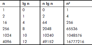
It can be observed from Table 2.1 that for a given input, the growth rate O(lg n) is faster than O(n lg n). For the same input size, the growth rate O(n2) is the slowest.
Later in the book, for various algorithms, timing estimates will be included using Big-Oh notation.
EXERCISES
- What is a stored program computer?
- Give the block diagram of Von Neumann architecture of a computer.
- What is a data structure? What is the need of data structures?
- List out the areas in which data structures are applied extensively. Why is it important to make a right choice of data structures for problem solving?
- What are built-in data structures? Give some examples.
- What are user-defined data structures? Give some examples.
- Consider a situation where it is required to rank 100 employees of an organization. The data of an employee consists of his name, designation, department, experience and salary. Give the possible choices for the data structures. Draw a comparison between the possible choices of organizing data.
- What is the difference between data type and data structure?
- Differentiate between linear and non-linear data structures. Explain with the help of examples.
- Explain the following basic terminologies associated with the data structures:
- Data element
- Primitive data types
- Data object
- Constant
- Variable
- What is an algorithm? Differentiate between algorithm and program.
- List the desirable features of an algorithm.
- What are the characteristics possessed by an algorithm?
- What are the steps that can be suggested for developing an algorithm? Consider a suitable scenario and develop an algorithm for solving the problem. Explain each step while developing the algorithm.
- What are the control structures? Explain the sequence control structures with the help of examples.
- Write an algorithm that computes area and perimeter of a rectangle.
- Write an algorithm that computes square of a number by repititive addition.
- Write an algorithm that computes GCD and LCM of two given numbers.
- Explain the selection (conditional control) structures with the help of examples.
- Write an algorithm that determines whether a number is even or odd.
- Write an algorithm that computes profit or loss incurred by a salesperson.
- What is iteration?
- Write an algorithm that sorts a given list of numbers in ascending order.
- Write an algorithm that determines whether a number is prime or not.
- What is the use of accumulators and counters?
- Write an algorithm that computes average marks of 60 students of a class.
- Write an algorithm that finds the number of odds and evens present in a given list of N numbers.
- What are the parameters on the basis of which an algorithm can be analyzed?
- Define the term ‘time complexity’. How can the time complexity of a given algorithm be found?
- Explain Big-Oh notation with the help of examples.
- Compute the time complexity of the following relations:
- T(n) = 410
- T(n) = 4*n − 12
- T(n) = 13*N2 − 7
- T(n) = 3*N3 + N2+4*N
- What is the time complexity of the following loop?
for (int i = 0; i < n; i++) { statement; } - What is the Big-Oh complexity of the following nested loop?
-
for (int i = 0; i < n; i++) { for (int j = 0; j < n; j++) { statement; } } -
for (int i = 0; i < n; i++) { for (int j = i + 1; j < n; j++) { statement; } } -
for (int i = 0; i < n; i++) { for (int j = n; j > i; j--) { statement; } } -
   for (int i = 0; i < n; i++)
   {
       for (int j = 0; j < m; j++)
       {
           statement1;
       }
           statement2;
   }
-
- Consider the following algorithm and compute its time complexity.
    if (a==b)
      statement1;
    else if (a > b)
      statement2;
    else
      statement3;