
Chapter 3
Arrays: Searching and Sorting
CHAPTER OUTLINE
3.1 INTRODUCTION
An array is a data structure with the help of which a programmer can refer to and perform operations on a collection of similar data types such as simple lists or tables of information. For example, a list of names of ‘N’ number of students of a class can be grouped under a common name (say studList). This list can be easily represented by an array called studList for ‘N = 45’ students as shown in Figure 3.1
In fact, the studList shown in Figure 3.1 can be looked upon by the following two points of views:
- It is a linear list of 45 names stored in contiguous locations—an abstract view of a list having finite number of homogeneous elements (i.e., 45 names).
- It is a set of 0 to 44 memory locations sharing a common name called studList—it is an array data structure in which 45 names have been stored.
It may be noted that all the elements in the array are of same type, i.e., string of char in this case. The individual elements within the array can be designated by an index. The individual elements are randomly accessible by integers, called the index.
For instance, the zeroth element (Sagun) in the list can be referred to as studList [0] and the 43rd element (Ridhi) as studList [43] where 0 and 43 are the indices. An index has to be of type integer.
An index is also called a subscript. Therefore, individual elements of an array are called subscripted variables. For instance, studList [0] and studList [43] are subscripted variables.
From the above discussion, we can define an array as a finite ordered collection of items of same type. It is a set of index, value pairs.
An array is a built-in data structure in every programming language. Arrays are designed to have a fixed size. Some languages provide zero-based indexing whereas other languages provide one-based indexing. ‘C’ is an example of zero-based indexing language because the index of its arrays starts from 0. Pascal is the example of one-based indexing because the index of its arrays starts from 1.
An array whose elements are specified by a single subscript is known as one-dimensional array. The array whose elements are specified by two or more than two subscripts is called as multi-dimensional array.
3.2 ONE-DIMENSIONAL ARRAYS
One-dimensional arrays are suitable for processing lists of items of identical types. They are very useful for problems that require the same operation to be performed on a group of data items. Consider Example 1.
Example 1: The examination committee of the university has decided to give 5 grace marks to every student of a class. Assume that there are 30 students in the class and their marks are stored in a list called ‘marksList’. Write a program that adds the grace marks to every entry in the ‘marksList’.
Solution: As the problem deals with a list of marks, we can select a one-dimensional array called ‘marksList’ to represent the list. The grace marks are to be added to all the elements of the list, for which we must use the For-loop. The required program is given below:
  /* This program adds grace marks to all elements of a list of marks */
  #include <stdio.h>
  void main()
  {
    int marksList[30];
    int i;
    int grace = 5;        /*grace marks */
    /* Read the marksList */
    printf (“
 Enter the list of marks one by one”);
    for (i = 0; i< 30; i++)
    {
        scanf (“%d”, &marksList[i]);
        marksList[i] = marksList[i] + grace;
    }
    /* Print the Final list */
    printf (“
 The final List is ...”);
    printf (“
 S. No.	 Marks”);
    for (i = 0; i < 30; i++)
     printf (“
 %d	%d”, i, marksList[i]);
  }
It may be noted that in the above program, a component by component processing has been done on the all elements of the array called marksList.
The following operations are defined on array data structure:
- Traversal: An array can be travelled by visiting its elements starting from the zeroth element to the last in the list.
- Selection: An array allows selection of an element for a given (random) index.
- Searching: An array can be searched for a particular value.
- Insertion: An element can be inserted in an array at a particular location.
- Deletion: An element can be deleted from a particular location of an array.
- Sorting: The elements of an array can be manipulated to obtain a sorted array.
We shall discuss the above–mentioned operations on arrays in the subsequent sections.
3.2.1 Traversal
It is an operation in which each element of a list, stored in an array, is visited. The travel proceeds from the zeroth element to the last element of the list. Processing of the visited element can be done as per the requirement of the problem.
Example 2: Write an algorithm called ‘listTravel’ that travels a list stored in an array called List of size N. Each visited element is operated upon by an operator called OP.
Solution: The For-loop can be employed to visit and apply the operator OP on every element of the array. The required algorithm is given below:
  Algorithm listTravel()
    {
     Step
      1. For (i = 0; i < N, i++)
       {
         1.1 List[i] = OP(List[i]);
       }
    }
Example 3: A list of N integer numbers is given. Write a program that travels the list and determines as to how many of the elements of the list are less than zero, zero, and greater than zero.
Solution: In this program, three counters called numNeg, numZero and numPos, would be used to keep track of the number of elements that are less than zero, zero, and greater than zero present in the list. The required program is given below:
  /* This program determines the number of less than zero, zero, and greater than zero numbers present in a list */

  #include <stdio.h>
  void main()
  {
   int List [30];
   int N;
   int i, numNeg, numZero, numPos;
    printf (“
 Enter the size of the list”);
    scanf (“%d”, &N);
    printf (“Enter the elements one by one”);
    /* Read the List*/
    for (i = 0; i < N; i++)
    {
     printf (“
 Enter Number:”);
     scanf (“%d”, &List[i]);
    }
    numNeg = 0; /* Initialize counters*/
    numZero = 0;
    numPos = 0;
    /* Travel the List*/
    for (i = 0; i < N; i++)
    {
       if (List[i] < 0)
          numNeg = numNeg + 1;
       else
         if (List[i] == 0)
          numZero = numZero + 1;
         else
         numPos = numPos + 1;
    }
  }
3.2.2 Selection
An array allows selection of an element for a given (random) index. Therefore, the array is also called random access data structure. The selection operation is useful in a situation wherein the user wants query about the contents of a list for a given position.
Example 4: Write a program that stores a merit list in an array called ‘Merit’. The index of the array denotes the merit position, i.e., 1st, 2nd, 3rd, etc. whereas the contents of various array locations represent the percentage of marks obtained by the candidates. On user’s demand, the program displays the percentage of marks obtained for a given position in the merit list as per the following format:
Position: 4
Percentage: 93.25
Solution: An array called ‘Merit’ would be used to store the given merit list. Two variables pos and percentage would be used to store the merit position and the percentage of a candidate, respectively. A do-while loop would be used to iteratively interact with the user through following menu displayed to the user:
Menu:
Query----1
Quit------2
Enter your choice
Note: As per the demand of the program, we will leave the zeroth location as unused and fill the array from index 1.
The required program is given below:
  /* This program illustrates the random selection operation allowed by array data structures */
  #include<stdio.h>
  #include<conio.h>
  void main()
  {
    float Merit[30];
    int size;
    int i;
    int pos;
    float percentage;
    int choice;
    printf (“
 Enter the size of the list”);
    scanf (“%d”, &size);
    printf (“
 Enter the merit list one by one”);
    for (i = 1; i < = size; i++) /* Read Merit */
    {
     printf (“
 Enter data:”);
     scanf (“%f”, &Merit[i]);
    }
     /* display menu and start session */
    do
    {
      clrscr();
      printf (“
 Menu”);
      printf (“
 Query--------1”);
      printf (“
 Quit --------2”);
      printf (“
 Enter your choice: ”);
      scanf (“%d”, & choice);
      /* use switch statement
      for determining the choice*/
      switch (choice)
      {
       case 1: printf(“
 Enter Position”);
        scanf(“%d”, &pos);
        percentage = Merit[pos]; /* the random selection */
        printf (“
 position = %d”, pos);
        printf (“
 percentage = %4.2f”,percentage);
        break;
       case 2: printf (“
 Quitting”);
      }
      printf (“
 press a key to continue...”);
      getch();
   }
     while (choice != 2);
  }
Searching and sorting are very important activities in a data processing environment and they are discussed in detail in the subsequent section.
3.2.3 Searching
There are many situations where we want to find out whether a particular item is present in a list or not. For instance, in a given voter list of a colony a person may search his name to ascertain whether he is a valid voter or not. For similar reasons, passengers look for their names in the railway reservation lists.
Note: System programs extensively search symbols, literals, mnemonics, ‘compiler and assembler’ directives, etc.
In fact, search is an operation in which a given list is searched for a particular value. The location of the searched element is informed. Search can be precisely defined an activity of looking for a value or item in a list.
A list can be searched sequentially wherein the search for the data item starts from the beginning and continues till the end of the list. This simple method of search is also called linear search. It may be noted that for a list of size 1,000, the worst case is 1,000 comparisons.
Let us consider a situation wherein we are interested in searching a list of numbers called ‘numList’ for an element having value equal to the contents of a variable called val. It is desired that the location of the element, if found, be displayed.
The list of numbers can be comfortably stored in an array called numList of type int. To find the element, the list would be travelled in such a manner that each visited element would be compared to the variable ‘val’. If the match is found, then the location of the corresponding position would be stored in a variable called Pos. As the number of elements in the list is known, For-loop would be used to travel the array.
  Algorithm searchList()
   {
    step
      1. read numList
      2. read Val
      3. Pos = −1 ’initialize Pos to a non-existing position’
      4. for (i = 0; i < N; i++)
        {
         4.1 if (val == numList[i])
                  Pos = i;
        }
      5. if (Pos != −1)
         print Pos.
  }
The ‘C’ implementation of the above algorithm is given below:
  /* This program searches a given value called Val in a list called numList */
  #include<stdio.h>
  void main()
  {
    int numList[20];
    int N; /* Size of the list*/
    int Pos, val, i;
    printf (“
 Enter the size of the List”);
    scanf (“%d”, &N);
    printf (“
 Enter the elements one by one”);
    for (i = 0; i < N; i++)
    {
     scanf (“%d”, &numList[i]);
    }
    printf (“
 Enter the value to be searched”);
    scanf (“%d”, &val);
                /* Search the element and its position in the list*/
    Pos = −1;
    for (i = 0; i < N; i++)
    {
      if (val== numList[i])
       {
        Pos = i;
        break;
       }
              /* The element is found – come out of loop*/
    }
    if (Pos != −1)
        printf (“
 The element found at %d location”, Pos);
    else
       printf (“
 Search Failed”);
  }
Example 5: Write a program that finds the second largest element in a given list of N numbers.
Solution: The most basic solution for this problem is that if there are two elements in the list then the smaller of the two will be the second largest. In this case, we would set the second largest number to ‘−9999’, a value not possible in the list.
In given problem, the list will be searched linearly for the required second largest number. Two variables called firstLarge and secLarge would be employed to store the first and second largest numbers. The following algorithm will be used:
  Algorithm SecLarge()
   {
       step
         1. read num;
         2. firstLarge = num;
         3. secLarge = -9999;
         4. for (i = 2; i < = N; i++)
           {
            4.1 read num;
            4.2 if (firstLarge < num)
               {secLarge = firstLarge;
               firstLarge = num;
           }
               else
               if (secLarge < num)
                   secLarge = num;
           }
         4. prompt "Second Large =”;
         5. write secLarge;
   }
The equivalent program is given below:
  /* This program finds the second largest in a given list of numbers */
  #include <stdio.h>
  int Num, firstLarge, secLarge;
  int N, i;
  void main()
  {
   printf (“
 Enter the size of the list”);
   scanf (“%d”, & N);
   printf (“
 Enter the list one by one”);
   scanf (“%d”, &Num);
   firstLarge = Num;
   secLarge = −9999;
   for (i = 2; i < = N; i++)
   {
      scanf (“%d”, &Num);
      if (firstLarge < Num)
      {secLarge = firstLarge;
      firstLarge = Num;
      }
      else
        if (secLarge < Num)
        secLarge = Num;
   }
      printf (“
 Second Large = %d”, secLarge);
  }
The above discussed search through a list, stored in an array, has the following characteristics:
- The search is linear.
- The search starts from the first element and continues in a sequential fashion from element to element till the desired entry is found.
- In the worst case, a total number of N steps need to be taken for a list of size N.
Thus, the linear search is slow and to some extent inefficient. In special circumstances, faster searches can be applied.
For instance, binary search is a faster method as compared to linear search. It mimics the process of searching a name in a directory wherein one opens a page in the middle of the directory and examines the page for the required name. If it is found, the search stops; otherwise, the search is applied either to first half of the directory or to the second half.
3.2.3.1 Binary Search
If a list is already sorted, then the search for an entry (say Val) in the list can be made faster by using ‘divide and conquer’ technique. The list is divided into two halves separated by the middle element as shown in Figure 3.2.
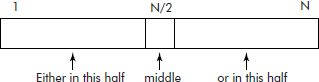
The binary search follows the following steps:
Step
- The middle element is tested for the required entry. If found, then its position is reported else the following test is made.
- If Val < middle, search the left half of the list, else search the right half of the list.
- Repeat step 1 and 2 on the selected half until the entry is found otherwise report failure.
This search is called binary because in each iteration, the given list is divided into two (i.e., binary) parts. Therefore, in next iteration the search becomes limited to half the size of the list to be searched. For instance, in first iteration the size of the list is N which reduces to almost N/2 in the second iteration and so on.
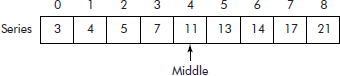
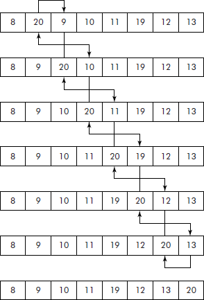
Let us consider a sorted list stored in an array called ‘Series’ given in Figure 3.3.
Suppose we desire to search the Series for a value (say 14) and its position in it. Binary search begins by looking at the middle value in the Series. The middle index of the array is approximated by averaging the first and last indices and truncating the result, i.e., (0 + 8)/2 = 4. Now, the content of the fourth location in Series happens to be ‘11’ as shown in Figure 3.4. Since the value we are looking for (i.e., 14) is greater than 11, the middle value, it may be present in the right half (Series [5] to Series [8]).
Now the middle of the right half is approximated i.e., (5 + 8)/2 = 6. We find that the desired element exists at the middle of the right half, i.e., Series [6] = 14 as shown in Figure 3.5.
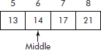
It may be noted that the desired element has been found only in two steps. Thus, it is a much faster method as compared to the linear search. For instance, a list of 1,000 sorted elements would require 10 comparisons to search the entire list. An algorithm for this method is given below.
In this algorithm, we would employ a Boolean variable called flag. The flag will indicate the presence or absence of the element being searched.
  Algorithm binSearch ()
    {
      Step
       1. First = 0;
       2. Last = N − 1;
       3. Pos =-1;
       4. Flag = false;
       5. While (First < = Last and Flag == false)
       {
          5.1 Middle = (first + last) div 2
             if (Series [middle] == Val)
              {Pos= middle;
              flag = true;
              break from the loop;
       }
             else
              if (Series[middle] < Val) First = middle + 1;
              else Last = middle − 1;
       }
       6. if (flag == true)
          prompt "The value found at”;
          write Val;
        else prompt "The value not found”;
    }
It may be noted that ‘div’ operator has been used to indicate that it is an integer division. The integer division will truncate the results to the nearest integer. If the desired value is found, then the flag is set to true and the while loop terminates; otherwise, a stage arrives when first becomes greater than the last, indicating the failure of the search. Thus, the variables First and Last keep track of the lower and the upper bounds of the array, respectively.
Example 6: Write a program that uses binary search to search a given value called Val in a list of N numbers called Series.
Solution: The Algorithm binSearch() discussed above is used to write the required program.
  /* This program uses binary search to find a given value called val in a list of N numbers */
  #include <stdio.h>
  #define true 1
  #define false 0
  void main()
  {
    int First;
    int Last;
    int Middle;
    int Series[20]; /*The list of N sorted numbers*/
    int Val;
    int flag; /*The value to be searched */
    int N, Pos, i;

    printf (“
 Enter the size of the list”);
    scanf (“%d”, & N);

    printf (“
 Enter the sorted list one by one”);

    for (i = 0; i< N; i++)
    {
        scanf (“%d”, &Series[i]);
    }
    printf (“
 Enter the number to be searched”);
    scanf (“%d”, & Val);
                        /* BIN SEARCH begins */
    Pos = −1;    /* Non-existing position */
    flag = false;       /* Assume search failure */

    First = 0;
    Last = N − 1;

      while ((First <= Last) && (flag == false))
      {
        Middle = (First + Last)/2;
        if (Series [Middle] == Val)
          {Pos = Middle;
           flag = true;
           break;
      }
      else
        if (Series[Middle] < Val)
        First = Middle + 1;
      else
        Last = Middle − 1;
      }
      if (flag == true)
        printf (“
 The value found at %d”, Pos);
      else
        printf (“
 The value not found”);
  }
Binary search through a list, stored in an array, has the following characteristics:
- The list must be sorted, i.e., ordered.
- It is faster as compared to the linear search.
- A list with large number of elements would increase the total execution time, the reason being that the list must be ordered which requires extra effort.
3.2.3.2 Analysis of Binary Search
As discussed above, we know that the binary search took two steps to search an element in a list of nine elements. However, in the worst case scenario for a list of 32 elements, we can visualize as follows:
Let us tabulate (Table 3.1) the number of steps taken by binary search for a given list of size n.
Table 3.1
| Size of list (n) | Number of steps | |
|---|---|---|
| 8 | (23) | 3 |
| 32 | (25) | 5 |
| 256 | (28) | 8 |
| 512 | (29) | 9 |
From table 3.1, we can infer that for a given input size n = 2k, number of steps =k.
Now the relation n = 2k can be rewritten as k = log2n (ax = n ≡ x = logan)
Thus, the time taken by binary search T(n) = k = log2n
To satisfy the relation 2.1, the above relation can be rewritten as shown below:
T(n) <= 1*log2n where c = 1 and n0 = 0.
Comparing the above relation with relation 2.1, we get g(n) = log2n. Therefore, the above relation can be expressed as:
T(n) = O(log2n)
Hence, binary search has time complexity of the order of log2n, i.e., O(log2n).
3.2.4 Insertion and Deletion
3.2.4.1 Insertion
Insertion is an operation in which a new element is added at a particular place in a list. When the list is represented using an array, the element can be added very easily at the end of the list provided the space is available. However, insertion of an element at a particular location within the list is a difficult operation. For instance, if it is desired to insert an element at ith location of a list then an empty space will have to be created at the ith location of the list. In fact, all the elements from ith location are shifted by one place towards right to accommodate the new element.
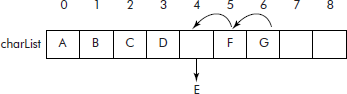
Consider a list of characters, represented using an array called ‘charList’ as shown in Figure 3.6. Suppose it is desired to insert a character ‘D’ at its proper place in charList, i.e., at the 3rd location.
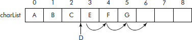
Now to accommodate the character ‘D’, the characters ‘G’, ‘F’, and ‘E’ will have to be shifted one step towards right to locations 6th, 5th, and 4th, respectively as per the operations shown below:
  charList [6] = charList[5];
  charList [5] = charList[4];
  charList [4] = charList[3];
Once the above copying operation is over, charList [3] becomes available for the storage of incoming character ‘D’ as shown below:
charList [3] = ’D’;
The array charList after the insertion operation is shown in Figure 3.7.
An algorithm for insertion of an element called val at ith location in an array called charList of size N is given below. Let us assume that the last element in the array is at Mth location. For instance, N = 8 and M = 5 in case of charList shown in Figure 3.6. A variable called Back is being used to point to the last empty location:
  Algorithm insertArray ()
   {
     Step
                  /* point to the last vacant position */
     1. if (M < N) then Back = M + 1;
      else
       STOP;
     2. while (Back > I);
      { /* Copy elements to next location in the list */
        2.1 charList [Back] = charList [Back − 1];
        2.2 Back = Back − 1;
      }
     3. charList [I] = val; /*Insert the element at ith location */
     4. M = M + 1;
   }
Example 7: Write a program that inserts an element called ‘key’ at a location called ‘loc’ in a list of M numbers called ‘List’.
Solution: The algorithm insertArray() is being used to implement the required program.
  /* This program inserts an element called Key into a list of numbers */
  #include <stdio.h>
  #define N 20
  void main()
  {
    int List[N];
    int Key;
    int Loc;
    int i, M;
    int back;

    printf (“
 Enter the size of the list (< 20)”);
    scanf (“%d”, &M);

    printf (“
 Enter the list one by one”);
    for (i = 0; i< M; i++)
    {
      scanf (“%d”, &List[i]);
    }
    printf (“
 Enter the key and location relative to 0 index”);
    scanf (“%d %d”, &Key, &Loc);
                   /* Insert the ’key’ at ’Loc’ in ’List’ */
    if (Loc > M + 1)
      printf (“
 Insertion not possible”);
    else
    {
     back = M + 1;
                /* Shift elements one step right */
     while (back > Loc)
     {
       List[back] = List [back − 1];
       back--;
     }
               /* Insert Key*/
       List[back] = Key;
       M=M + 1;
                /* Display the final list */
       printf (“
 The Final List is ......”);
       for (i = 0; i < M; i++)
      {
       printf (“%d ”, List[i]);
      }
    }
  }
3.2.4.2 Deletion
Deletion is the operation that removes an element from a given location of a list. When the list is represented using an array, the element can be very easily deleted from the end of the list. However, if it is desired to delete an element from an ith location of the list, then all elements from the right of (i+1)th location will have to be shifted one step towards left to preserve contiguous locations in the array.
For instance, if it is desired to remove an element from 4th location of the list given in Figure 3.8, then all elements from right of 4th location would have to be shifted one step towards left.
Now to delete the character ‘E’, the characters ‘F’ and ‘G’ will have to be shifted one step towards left to locations 4th and 5th, respectively as per the operations shown below:
  charList [4] = charList[5];
  charList [5] = charList[6];
It may be noted that the contents of charList [5] (i.e., ‘F’) overwrites the contents of charList [4] (i.e., E). The array charList after the deletion operation is shown in Figure 3.9.
An algorithm for deletion of an element from ith location in an array called charList of size N is given below. Let us assume that the last element in the array is at Mth location. For instance, N = 8 and M = 6 in case of charList shown in Figure 3.8. A variable called Back is used to point to the last empty location.
  Algorithm delElement()
  {
    Step
      1. Back = I; /* point to the location from where deletion is desired */
      2. while (Back < M)
      {
        2.1 charList[Back] = charList[Back + 1];        /* Shift    elements one
            step left*/
        2.2 Back = Back + 1;
      }
      3. M = M − 1;
      4. Stop
  }
It may be noted that in step 3, the contents of M have been decremented by 1 to indicate that after deletion the last element in the charList would be at (M – 1)th location.
Example 8: Write a program that deletes an element from a location called loc in a list of M numbers called ’List’.
Solution: The algorithm delElement() is used to implement the required program.
  /*This program deletes an element from list of numbers */
  #include <stdio.h>
  #define N 20
  void main()
  {
    int List[N];
    int Loc;
    int i, M;
    int back;
    printf (“
 Enter the size of the list (< 20)”);
    scanf (“%d”, &M);
    printf (“
 Enter the list one by one”);
    for (i = 0; i< M; i++)
    {
       scanf (“%d”, &List[i]);
    }
    printf (“
 Enter location from where the deletion is required”);
    scanf (“%d”, &Loc);
                /* Insert the ’key’ at ’Loc’ in ’List’ */
    if (Loc > M)
       printf (“
 Deletion not possible”);
    else
    {
      back = Loc;
             /* Shift elements one step left */
      while (back < M)
      {
        List[back] = List [back + 1];
        back++;
      }
      M=M − 1;
                   /* Display the final list */
      printf (“
 The Final List is ......”);
      for (i = 0; i < M; i++)
      {
       printf (“%d ”, List[i]);
      }
    }
  }
It may be noted that arrays are not suitable data structures for problems requiring insertions and deletions in a list. The reason is that we need to shift elements to right or to left for insertion and deletion operations, respectively. The problem aggravates when the size of the list is very large as an equally large number of shift operations would be required to insert and delete the elements. Thus, insertion and deletion are very slow operations as far as arrays are concerned.
3.2.5 Sorting
It is an operation in which all the elements of a list are arranged in a predetermined order. The elements can be arranged in a sequence from smallest to largest such that every element is less than or equal to its next neighbour in the list. Such an arrangement is called ascending order. Assuming an array called List containing N elements, the ascending order can be defined by the following relation:
List[i] <= List [i + 1], 0 < i < N – 1
Similarly in descending order, the elements are arranged in a sequence from largest to smallest such that every element is greater than or equal to its next neighbour in the list. The descending order can be defined by the following relation:
List[i] >= List [i + 1] , 0 < i < N – 1
It has been estimated that in a data processing environment, 25 per cent of the time is consumed in sorting of data. Many sorting algorithms have been developed. Some of the most popular sorting algorithms that can be applied to arrays are in-place sort algorithms. An in-place algorithm is generally a comparison-based algorithm that stores the sorted elements of the list in the same array as occupied by the original one. A detailed discussion on sorting algorithms is given in subsequent sections.
3.2.5.1 Selection Sort
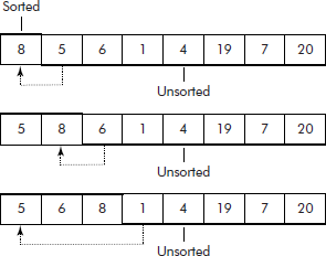
It is a very simple and natural way of sorting a list. It finds the smallest element in the list and exchanges it with the element present at the head of the list as shown in Figure 3.10.
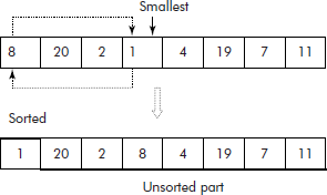
It may be noted from Figure 3.10 that initially, whole of the list was unsorted. After the exchange of smallest with the element on the head of the list, the list is divided into two parts: sorted and unsorted.
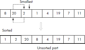
Now the smallest is searched in the unsorted part of the list, i.e., ‘2’ and exchanged with the element at the head of unsorted part, i.e., ‘20’ as shown in Figure 3.11.
This process of selection and exchange (i.e., a pass) continues in this fashion until all the elements in the list are sorted (see Figure 3.12). Thus, in selection sort, two steps are important—selection and exchange.
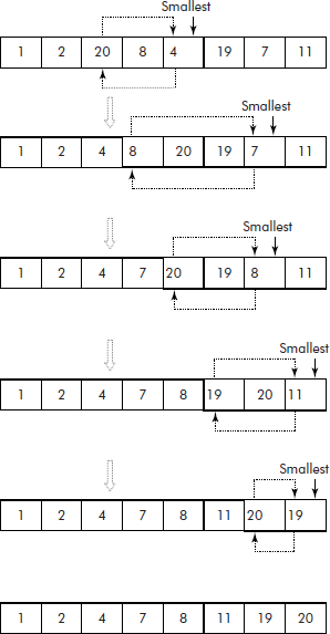
From Figures 3.11 and 3.12, it may be observed that it is a case of nested loops. The outer loop is required for passes over the list and the inner loop for searching smallest element within the unsorted part of the list. In fact, for N number of elements, N − 1 passes are made.
An algorithm for selection sort is given below. In this algorithm, the elements of a list stored in an array called LIST[N] are sorted in ascending order. Two variables called Small and Pos are used to locate the smallest element in the unsorted part of the list. Temp is the variable used to interchange the selected element with the first element of the unsorted part of the list.
  Algorithm SelSort()
   {
     Step
       1. For I = 1 to N − 1 /* Outer Loop */
     {
       1.1 small = List [I];
       1.2 Pos = I;
       1.3 For J = I + 1 to N /* Inner Loop */
       {
         1.3.1 if (List [J] < small)
         {
           small = List[J];
           Pos = J; /* Note the position of the smallest*/
         }
     }
       1.4 Temp = List [I]; /*Exchange smallest with the Head */
       1.5 List [I] = List [Pos];
       1.6 List [Pos] = Temp;
     }
     2. Print the sorted list
   }
Example 9: Given is a list of N randomly ordered numbers. Write program that sorts the list in ascending order by using selection sort.
Solution: The required program is given below:
In this program, the elements of a list are stored in an array called List. The elements are sorted using above given Algorithm selSort(). Two variables small and pos have been used to locate the smallest element in the unsorted part of the list. Temp is a variable used to interchange the selected element with the first element of the unsorted part of the list. With each step, the unsorted part becomes smaller. The process is repeated till all the elements are sorted.
  /* This program sorts a list by using selection sort */
  #include <stdio.h>
  main()
  {
    int list [10];
    int small, pos, N, i, j, temp;
    printf (“
 Enter the size of the list:”);
    scanf (“%d”, & N);

    printf (“
 Enter the list: ”);
    for (i = 0; i < N; i++)
    {
      printf (“
 Enter Number:”);
      scanf (“%d”, &list[i]);
    }
                  /* Sort the list */
    for (i = 0; i < N − 1; i++)
    {
      small = list[i];

      pos = i;

                   /* Find the smallest of the unsorted list */
      for (j = i+1; j < N; j++)
      {
        if (small > list [j])
        {
          small = list [j];
          pos = j;
        }
      }
                   /* Exchange the small with the first element of unsorted list */
      temp = list [i];
      list [i] = list [pos];
      list [pos] = temp;
    }
    printf (“
 The sorted list ...”);
    for (i = 0; i < N; i++)
    printf (“%d ”, list[i]);
  }
3.2.5.2 Analysis of Selection Sort
In selection sort, there are two major operations: comparison and exchange. The average number of exchange operations would be difficult to estimate. Therefore, we will focus on comparison operations.
It may be noted that for every execution of outer loop, the inner loop executes in decreasing order. For example, in a list of (say) eight numbers, the first number would be compared to the remaining seven numbers to find out the smallest. After bringing the smallest to the first position, the second number would be compared to the remaining six, the third number with remaining five, and so on. Thus, the total number of comparisons for a list on N elements would be:
(N − 1) + (N − 2) + …….2 + 1 = (N − 1) N/2 = N2/2 − N/2
Thus, T(n) = N2/2 − N/2.
we can say that
N2/2 − N/2 <= N2/2.
Therefore, we can say that
T(n) <= N2/2 where c = ½ , n0 = 0 , g(n) = N2
T(n) = O(N2)
Hence, selection sort has time complexity of the order of N2, i.e., O(N2).
3.2.5.3 Bubble Sort
It is also a very simple sorting algorithm. It proceeds by looking at the list from left to right. Each adjacent pair of elements is compared. Whenever a pair is found not to be in order, the elements are exchanged. Therefore after the first pass, the largest element bubbles up to the right end of the list. A trace of first pass on a list of numbers is shown in Figure 3.13.
It may be noted that after the pass is over, the largest element in the list (i.e., 20) has bubbled up to the end of the list and six exchanges were made. Now the same process can be repeated for the list for second pass as shown in Figure 3.14.
We observe that after the second pass is over, the list has become sorted and only two exchanges were made. Now a point worth noting is as to how and when it will be decided that the list has become sorted. The simple criteria would be to check whether or not any exchange(s) has been made during the current pass. If ‘yes’, then the list is not yet sorted otherwise if it is ‘no’, then it can be decided that the list has just become sorted.
An algorithm for bubble sort is given below. In this algorithm, the elements of a list, stored in an array called List[N], are sorted in an ascending order. The algorithm uses two loops—the outer while loop and inner For loop. The inner For loop makes a pass on the list. If during the pass, any exchange(s) is made then it is recorded in a variable called flag, i.e., flag is set to false. The outer while loop keeps track of the flag. As soon as the flag informs that no exchange(s) took place during the current pass indicating that the list is now sorted, the algorithm stops.
  Algorithm bubbleSort()
  {
    Step
    1. Flag = false;
    2. While (Flag == false)
    {
     2.1 Flag = true;
     2.2 For j = 0 to N − 2
     {
       2.2.1 if (List [J] > List [J + 1])
       {
          temp = List[J];
          List[J] = List [J + 1];
          List [J + 1] = temp;
          Flag=false;
        }
      }
    }
    3. Print the sorted list
    4. Stop
  }
It may be noted that the algorithm stops as soon as the list becomes sorted. Thus, ‘bubble sort’ is a very useful algorithm when the list is almost sorted i.e., only a very small percentage of elements are out of order.
Example 10: Given is a list of N randomly ordered numbers. Write a program that sorts the list in ascending order by using bubble sort.
Solution: The required program is given below:
In this program, the elements of a list are stored in an array called List. The elements are sorted using above given algorithm bubbleSort().
  / *This program sorts a given list of numbers in ascending order, using bubble sort */
  #include <stdio.h>
  #define N 20
  #define true 1
  #define false 0
  void main()
  {
    int List[N];
    int flag;
    int size;
    int i, j, temp;
    int count; /* counts the number of passes*/
    printf (“
 Enter the size of the list (< 20)”);
    scanf (“%d”, &size);
    printf (“
 Enter the list one by one”);
    for (i = 0; i< size; i++)
    {
      scanf (“%d”, &List[i]);
    }
             /* Sort the list by bubble sort */
    flag = false;
    count = 0;
    while (flag == false)
    {
       flag = true; /* Assume no exchange takes place*/
       count++;
       for (j =0; j< size−1; j++)
       {
         if (List[j] > List[j+1])
         {     /* Exchange the contents */
           temp = List[j];
           List[j] = List[j + 1];
           List[j + 1] = temp;
           flag = false; /* Record the exchange operation*/
         }
       }
    }
               /* Print the sorted list*/
        printf (“
 The sorted list is ....”);
        for (i = 0; i< size; i++)
         printf (“%d ”, List[i]);
        printf (“
 The number of passes made = %d”, count);
  }
It may be noted that the above program has used a variable called count that counts the number of passes made while sorting the list. The test runs conducted on the program have established that the program is very efficient in case of almost sorted list of elements. In fact, it takes only one scan to establish that the supplied list is already sorted.
Note: Bubble sort is also called a sinking sort meaning that the elements sink down in the list to their proper position.
3.2.5.4 Analysis of Bubble Sort
In bubble sort, again, there are two major operations—comparison and exchange. The average number of exchange operations would be difficult to estimate. Therefore, we will focus on comparison operations.
A closer look reveals that for a list of N numbers, bubble sort also has the following number of comparisons, i.e., same as the selection sort.
(N – 1) + (N – 2) + ……. 2 + 1 = (N – 1) N/2 = N2/2 – N/2
Therefore, the time complexity of bubble sort is also O(N2).
However if the list is already sorted in the ascending order, no exchange operations would be required and it becomes the best case. The algorithm will have only N comparisons, i.e., only a linear running time.
3.2.5.5 Insertion Sort
This algorithm mimics the process of arranging a pack of playing cards. In the pack of cards, the first two cards are put in correct relative order. The third card is inserted at correct place relative to the first two. The fourth card is inserted at the correct place relative to the first three, and so on.
Given a list of numbers, it divides the list into two part—sorted part and unsorted part. The first element becomes the sorted part and the rest of the list becomes the unsorted part as shown in Figure 3.15. It picks up one element from the front of the unsorted part and inserts it at its proper position in the sorted part of the list. This insertion action is repeated till the unsorted part is exhausted.
It may be noted that the insertion operation requires following steps:
Step
- Scan the sorted part to find the place where the element, from unsorted part, can be inserted. While scanning, shift the elements towards right to create space.
- Insert the element, from unsorted part, into the created space.
The algorithm for the insertion sort is given below. In this algorithm, the elements of a list stored in an array called List[N] are sorted in an ascending order. The algorithm uses two loops—the outer For loop and inner while loop. The inner while loop shifts the elements of the sorted part by one step to right so that proper place for incoming element is created. The outer For loop inserts the element from unsorted part into the created place and moves to next element of the unsorted part.
  Algorithm insertSort()
  {
    Step
     1. For I = 2 to N /* The first element becomes the sorted part */
      {
      1.1 Temp = List [I]; /* Save the element from unsorted part into temp */
      1.2 J = I − 1;
      1.3 While (Temp < = List [J] AND J > = 0)
        {
          List[J + 1] = List[J]; /* Shift elements towards right */
          J = J - 1;
        }
      1.4 List [J + 1] = Temp;
      }
     2. Print the list
     3. Stop
  }
Example 11: Given is a list of N randomly ordered numbers. Write a program that sorts the list in ascending order by using insertion sort.
Solution: The required program is given below:
  /*This program sorts a given list of numbers in ascending order using insertion sort */
  #include <stdio.h>
  #define N 20
  void main()
  {
    int List[N];
    int size;
    int i, j, temp;
    printf (“
 Enter the size of the list (< 20)”);
    scanf (“%d”, &size);
    printf (“
 Enter the list one by one”);
    for (i = 0; i < size; i++)
    {
      scanf (“%d”, &List[i]);
    }
                  /* Sort the list by Insertion sort */
    for (I=1; i<size; i++)
    {
      temp = List[i]; /* Pick and save the first element of the unsorted
      part*/
      j= i - 1;
      while ((temp < List[j])&& (j>=0)) /* Scan for proper place */
      {
        List[j + 1] = List[j];
        j = j - 1;
      }
        List[j+1] = temp; /* Insert the element at the proper place */
     }
     /* Print the sorted list*/
     printf (“
 The sorted list is ....”);
     for (i = 0; i< size; i++)
     {
      printf (“%d ”, List[i]);
     }
  }
3.2.5.6 Analysis of Insertion Sort
A critical look at the algorithm indicates that in worst case, i.e., when the list is sorted in reverse order, the jth iteration requires (j − 1) comparisons and copy operations. Therefore, the total number of comparison and copy operations for a list of N numbers would be:
1 + 2 + 3 +…….(N – 2) + (N – 1) = (N – 1) N/2 = N2/2 – N/2
Therefore, the time complexity of insertion sort is also O(N2).
However if the list is already sorted in the ascending order, no copy operations would be required. It becomes the best case and the algorithm will have only N comparisons, i.e., a linear running time.
3.2.5.7 Merge Sort
This method uses following two concepts:
- If a list is empty or it contains only one element, then the list is already sorted. A list that contains only one element is also called singleton.
- It uses the old proven technique of ‘divide and conquer’ to recursively divide the list into sub-lists until it is left with either empty or singleton lists.
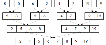
In fact, this algorithm divides a given list into two almost equal sub-lists. Each sub-list, thus obtained, is recursively divided into further two sub-lists and so on till singletons or empty lists are left as shown in Figure 3.16.
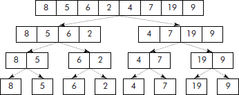
Since the singletons and empty lists are inherently sorted, the only step left is to merge the singletons into sub-lists containing two elements each (see Figure 3.17) which are further merged into sub-lists containing four elements each and so on. This merging operation is recursively carried out till a final merged list is obtained as shown in Figure 3.17.
Note: The merge operation is a time consuming and slow operation. The working of merge operation is discussed in the next section.
Merging of lists It is an operation in which two ordered lists are merged into a single ordered list. The merging of two lists PAR1 and PAR2 can be done by examining the elements at the head of the two lists and selecting the smaller of the two. The smaller element is then stored into a third list called mergeList. For example, consider the lists PAR1 and PAR2 given in Figure 3.18. Let Ptr1, Ptr2, and Ptr3 variables point to the first locations of lists PAR1, PAR2, and PAR3, respectively. The comparison of PAR1[Ptr1] and PAR2[Ptr2] shows that the element of PAR1 (i.e., ‘2’) is smaller. Thus, this element will be placed in the mergeList as per the following operation:
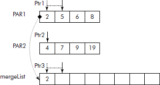
  mergeList[Ptr3] = PAR1[Ptr1];
  Ptr1++;
  Ptr3++;
Since an element from the list PAR1 has been taken to mergeList, the variable Ptr1 is accordingly incremented to point to the next location in the list. The variable Ptr3 is also incremented to point to next vacant location in mergeList.
This process of comparing, storing and shifting is repeated till both the lists are merged and stored in mergeList as shown in Figure 3.19.
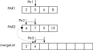
It may be noted here that during this merging process, a situation may arise when we run out of elements in one of the lists. We must, therefore, stop the merging process and copy rest of the elements from unfinished list into the final list.
The algorithm for merging of lists is given below. In this algorithm, the two sub-lists are part of the same array List[N]. The first sub-list is stored in locations List[lb] to List[mid] and the second sub-list is stored in locations List [mid+1] to List [ub] where lb and ub mean lower and upper bounds of the array, respectively.
  Algorithm merge (List, lb, mid, ub)
  {
      Step
        1. ptr1 = lb; /* index of first list */
        2. ptr2 = mid; /* index of second list */
        3. ptr3 = lb; /* index of merged list */
        4. while ((ptr1 <mid) && ptr2 < = ub) /* merge the lists */
         {
         4.1 if (List[ptr1] < = List [ptr2])
            {mergeList [ptr3] = List[ptr1]; /* element from first list is taken */
            ptr1++; /* move to next element in the list*/
            ptr3++;
         }
         4.2 else
             {mergeList [ptr3] = List[ptr2]; /* element from second list is taken*/
             ptr2++; /* move to next element in the list*/
             ptr3++;
          }
          }
        5. while (ptr1 < mid) /* copy remaining first list */
          {
          5.1 mergeList [ptr3] = List[ptr1];
          5.2 ptr1++;
          5.3 ptr3++;
          }
        6. while (ptr2 <= ub) /* copy remaining second list */
          {
          6.1 mergeList [ptr3] = List[ptr2];
          6.2 ptr2++;
          6.3 ptr3++;
          }
        7. for (i = lb; i<ptr3; i++) /* copy merged list back into original list */
          7.1 List[i] = mergeList[i];
        8. Stop
  }
It may be noted that an extra temporary array called mergeList is required to store the intermediate merged sub-lists. The contents of the mergeList are finally copied back into the original list.
The algorithm for the merge sort is given below. In this algorithm, the elements of a list stored in an array called List[N] are sorted in an ascending order. The algorithm has two parts—mergeSort and merge. The merge algorithm, given above, merges two given sorted lists into a third list, which is also sorted. The mergeSort algorithm takes a list and stores into an array called List[N]. It uses two variables lb and ub to keep track of lower and upper bounds of list or sub-lists as the case may be. It recursively divides the list into almost equal parts till singletons or empty lists are left. The sub-lists are recursively merged through merge algorithm to produce final sorted list.
  Algorithm mergeSort (List, lb, ub)
    {
      Step
        1. if (lb < ub)
        {
         1.1 mid = (lb + ub)/2; /* divide the list into two sub-lists */
         1.2 mergeSort (List, lb, mid); /* sort the left sub-list */
         1.3 mergeSort (List, mid +1, ub); /* sort the right sub-list */
         1.4 merge(List, lb,mid+1,ub); /* merge the lists */
        }
        2. Stop
    }
Example 12: Given is a list of N randomly ordered numbers. Write a program that sorts the list in ascending order by using merge sort.
Solution: The required program uses both the algorithms—mergeSort() and merge().
  /* This program sorts a given list of numbers in ascending order using merge sort */
  #include <stdio.h>
  #include <conio.h>
  #define N 20
  void mergeSort (int List[], int lb, int ub);
  void merge (int List[], int lb, int mid, int ub);
  void main()
  {
    int List[N];
    int i, size;
    int mid;
    printf (“
 Enter the size of the list (< 20)”);
    scanf (“%d”, &size);
    printf (“
 Enter the list one by one”);
    for (i=0; i< size; i++)
    {
      scanf (“%d”, &List[i]);
    }
              /* Sort the list by merge sort */
    mergeSort (List,0,size − 1);
    printf (“
 The sorted list is ....”);
    for (i = 0; i< size; i++)
    {
      printf (“%d ”, List[i]);
    }
  }
  void mergeSort (int List[], int lb, int ub)
  {
    int mid;
    if (lb < ub)
    {
      mid = (lb + ub)/2;
      mergeSort (List, lb, mid);
      mergeSort (List, mid + 1, ub);
      merge(List, lb, mid + 1,ub);
    }
  }
  void merge (int List[], int lb, int mid, int ub)
  {
    int mergeList[20];
    int ptr1, ptr2, ptr3;
       int i;
    ptr1=lb;
    ptr2=mid;
    ptr3=lb;
    while ((ptr1 <mid) && ptr2 < = ub)
    {
     if (List[ptr1] < = List [ptr2])
     {mergeList [ptr3] = List[ptr1];
     ptr1++;
     ptr3++;
     }
     else
     {mergeList [ptr3] = List[ptr2];
     ptr2++;
     ptr3++;
     }
    }
    while (ptr1 < mid)
    {mergeList [ptr3] = List[ptr1];
    ptr1++;
    ptr3++;
    }
    while (ptr2 <= ub)
    {mergeList [ptr3] = List[ptr2];
    ptr2++;
    ptr3++;
    }
    for (i = lb; i<ptr3; i++)
    {
      List[i] = mergeList[i];
    }
  }
3.2.5.8 Analysis of Merge Sort
The merge sort requires the following operations:
- Divide the list into two sub-lists.
- Sort each sub-list.
- Merge the two sub-lists.
- If number of elements = 1, then list is sorted.
For a list of N elements, steps 1 and 2 require two times the number of comparisons needed for sorting a sub-list of size N/2. The step 3 requires N steps to merge the two sub-lists.
Therefore, number of comparisons in merge sort can be defined by the following recursive relation:
NumComp (N) = 0 if N = 1,
= 2*NumComp(N/2) + N for N > 1
Thus, NumComp (1) = 0
By similarity, we can define the following:
NumComp (N/2) = 2*NumComp(N/4) + N
Putting above expressions into Eq. 3.1, we get
By repeating the above pattern, we shall arrive at the following relation:
We can generalize the above relation as:
The merge sort stops when we are left with one element per partition, i.e., when N= 2k.
Now for N = 2k or k = log2N, we can rewrite Eq. 3.4 as:
NumComp (N) = N NumComp(N/N) + N*log2N
= N NumComp(1) + N*log2N = N*0 + log2N*N = N*log2N
= N*log2N
Thus, T(N) = N*log2N <= C*N*log2N + n0
T(N) = O(N*log2N) for c = 1 and n0 = 0
Thus, the time complexity of merge sort is of the order of N*log2N or simply n log n.
3.2.5.9 Quick Sort
This method also uses the technique of ‘divide and conquer’. On the basis of a selected element (pivot) from of the list, it partitions the rest of the list into two parts—a sub-list that contains elements less than the pivot and other sub-list containing elements greater than the pivot. The pivot is inserted between the two sub-lists. The algorithm is recursively applied to the sub-lists until the size of each sub-list becomes 1, indicating that the whole list has become sorted.
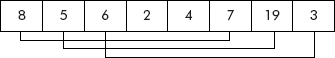
Consider the list given in Figure 3.20. Let the first element (i.e., 8) be the pivot. Now the rest of the list can be divided into two parts—a sub-list that contains elements less than ‘8’ and the other sub-list that contains elements greater than ‘8’ as shown in Figure 3.20.
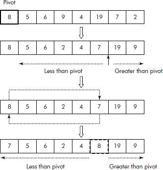
Now this process can be recursively applied on the two sub-lists to completely sort the whole list. For instance, ‘7’ becomes the pivot for left sub-list and ‘19’ becomes pivot for the right sub-list.
Note: Two sub-lists can be safely joined when every element in the first sub-list is smaller than every element in the second sub-list. Since ‘join’ is a faster operation as compared to a ‘merge’ operation, this sort is rightly named as a ‘quick sort’.
The algorithm for the quick sort is given below:
In this algorithm, the elements of a list, stored in an array called List[N], are sorted in an ascending order. The algorithm has two parts—quickSort and partition. The partition algorithm divides the list into two sub-lists around a pivot. The quickSort algorithm takes a list and stores it into an array called List[N]. It uses two variables lb and ub to keep track of lower and upper bounds of list or sublists as the case may be. It employs partition algorithm to sort the sub-lists.
  Algorithm quickSort()
  {
     Step
      1. Lb = 0; /*set lower bound */
      2. ub = N − 1; /* set upper bound */
      3. pivot = List [lb];
      4. lb++;
      5. partition (pivot, List, lb, ub);
  }
  Algorithm partition (pivot, List, lb, ub)
  {
    Step
      1. i = lb;
      2. j = ub;
      3. while (i<=j)
       {
                    /* travel the list from lb till an element greater than the pivot is found */
       3.1 while (List[i] <= pivot) i++;
                    /* travel the list from ub till an element smaller than the pivot is found */
       3.2 while (List[j] > pivot) j−−;
       3.3 if (i < = j) /* exchange the elements */
         {
         temp = List[i];
         List[i] = List[j];
         List[j] = temp;
         }
       }
      4. temp = List[j]; /* place the pivot at mid of the sub-lists */
      5. List[j] = List[lb − 1];
      6. List[lb − 1] = temp;
      7. if (j > lb) quicksort (List, lb, j − 1); /* sort left sub-       list */
      8. if (j < ub) quicksort (List, j + 1,ub); /* sort the right sub-list */
  }
Example 13: Given is a list of N randomly ordered numbers. Write a program that sorts the list in ascending order by using quick sort.
Solution: The required program uses both the algorithms—quickSort() and partition(). In this program, a variable called Key has been used that acts as a pivot.
  /* This program sorts a given list of numbers in ascending order, using quick sort */
  #include <stdio.h>
  #include <conio.h>
  #define N 20
  void partition (int Key, int List[], int lb, int ub);
  void quicksort (int List[], int lb, int ub);
  void main()
  {
    int List[N];
    int i, size, Pos, temp;
    int lb, ub;

    printf (“
 Enter the size of the list (< 20)”);
    scanf (“%d”, &size);

    printf (“
 Enter the list one by one”);
    for (i = 0; i < size; i++)
    {
     scanf (“%d”, &List[i]);
    }
                /* Sort the list by quick sort */
    quicksort (List, 0, size − 1);
                /* Print the sorted list*/
    printf (“
 The sorted list is ....”);
    for (i = 0; i< size; i++)
    {
     printf (“%d ”, List[i]);
    }
  }

  void quicksort (int List[], int lb, int ub)
  {
    int Key; /* The Pivot */
    Key =List [lb]; lb++;
    partition (Key, List, lb, ub);
  }

  void partition (int Key, int List[], int lb, int ub)
  {
    int i, j, temp;
    i = lb;
    j = ub;
      while (i<=j)
      {
      while (List[i] <= Key) i++;
      while (List[j] > Key) j−−;
      printf(“
i=%d j=%d”, i, j);
      getch();
      if (i <=j)
      {
      temp = List[i];
      List[i] = List[j];
      List[j] = temp;
      }
    }
    temp = List[j];
    List[j] = List[lb − 1];
    List[lb − 1] = temp;
    if (j > lb) quicksort (List, lb, j − 1);
    if (j < ub) quicksort (List, j + 1, ub);
  }
3.2.5.10 Analysis of Quick Sort
The quick sort requires the following operations:
Step
- If number of elements = 1, then list is sorted and exit.
- Partition the list into two sub-lists around a pivot.
- Place pivot in the middle of two sub-lists.
- Repeat steps 1 to 3.
The best case for quick sort algorithm comes when we split the input as evenly as possible into two sub-lists. Thus in the best case, each sub-list would be of size n/2. Anyway, the partitioning operation would require N comparisons to split the list of size N into the required sub-lists.
Now, for a list of size N, the number of comparisons can be defined as follows:
NumComp(N) = 0 when N = 1
= N + NumComp(sub-list1 of size N/2) + NumComp(sub-list2 of size N/2)
= N + 2*NumComp(N/2)
The above relation is same as defined in merge sort; therefore, it can be deduced to the following:
T(N) = O(N*log2N)
Thus, the best case time complexity of quicksort is of the order Nlog2N or simply n log n.
3.2.5.11 Shell Sort
It is an improvement on insertion sort. Given a list of List[N], it is divided into k sets of N/k items each. k can assume values from a set {1, 3, 5, 19, 41…}. Thus, the ith set will have the following elements:
Set i = List[i] List[i + k] List[i + 2k] …
Consider the list given in Figure 3.21.
For k = 5, the list is divided into the following sets:
Set 0 = 8, 7
Set 1 = 5, 19
Set 3 = 2
Set 4 = 4
Now on each set, the insertion sort is applied resulting in the arrangement shown in Figure 3.22. For k = 3, the list is divided into the following sets:
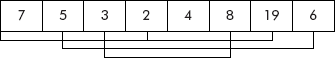
Set 0 = 7, 2, 19
Set 1 = 5, 4, 6
Set 2 = 3, 8
Now on each set, the insertion sort is applied resulting into the arrangement shown in Figure 3.23.
For k = 1, the list is represented by the following set:
Set 0 = 2, 4, 3, 7, 5, 8, 19, 6
Application of insertion sort on the above set results in the arrangement shown in Figure 3.24
It may be noted that the list is now sorted after the third pass. Since the variable k takes the diminishing values—5, 3, and 1; the shell sort is also called diminishing step sort.
The algorithm for the shell sort is given below. In this algorithm, a list of elements, stored in an array called List[N], are sorted in an ascending order. The algorithm divides the list into sets as per the description given above. The diminishing step values are stored in a list called dimStep. A variable ‘s’ is used that moves the insertion operation to the next set. The variable k takes the step size from dimStep and moves the index i within the set from one element to another.
  Algorithm shellSort()
  {
     Step
       1. initialize the set dimStep to values 1,3,5,...
                      /* sort the list by shell sort */
       2. for (step =0; step <3; step++)
       {
         2.1 k = dimStep[step]; /* set k to diminishing step */
         2.2 s = 0; /* start from the set of the list */
         2.3 for (i = s + k; i <size; i + = k)
           {
           temp = List[i]; /* save the element from the set */
           j = i − k;
                       /* find the place for insertion */
           while ((temp <List[j]) && (j > = 0))
           {
             List[j + k] = List[j];
             j = j − k;
           }
             List[j + k] = temp; /* insert the saved element at its place */
             s++; /* go to next set */
           }
       }
       3. print the sorted list
       4. Stop
  }
Example 14: Given is a list of N randomly ordered numbers. Write a program that sorts the list in ascending order by using shell sort.
Solution: The required program uses the algorithm shellSort().
  /* This program sorts a given list of numbers in ascending order using Shell sort */
  #include <stdio.h>
  #define N 20
  void main()
  {
    int List[N];
    int size;
    int i, j, k, p;
    int temp, s, step;
    int dimStep[] = {5,3,1}; /* the diminishing steps */
    printf (“
 Enter the size of the list (< 20)”);
    scanf (“%d”, &size);
    printf (“
 Enter the list one by one”);
    for (i=0; i< size; i++)
    {
      scanf (“%d”, &List[i]);
    }
                /* sort the list by shell sort */
    for (step =0; step <3; step++)
    {
      k = dimStep[step]; /* set k to diminishing step */
      s=0; /* start from the set of the list */
      for (i = s + k; i <size; i += k)
    {
      temp = List[i]; /* save the element from the set */
      j=i − k;
      while ((temp <List[j]) && (j >=0)) /* find the place for insertion       */
      {
        List[j + k] = List[j];
        j = j − k;
      }
      List[j + k] = temp; /* insert the saved element at its place */
      s++; /* go to next set */
     }
    }                      /* Print the sorted list*/
    printf (“
 The sorted list is ....”);
    for (i = 0; i< size; i++)
    {
        printf (“%d ”, List[i]);
    }
  }
The analysis of shell sort is beyond the scope of the book.
3.2.5.12 Radix Sort
It is a non-comparison-based algorithm suitable for integer values to be sorted. It sorts the elements digit by digit. It starts sorting the elements according to the least significant digit of the elements. This partially sorted list is then sorted on the basis of second least significant bit and so on.
Note: This algorithm is suitable to be implemented through linked lists. Therefore, discussion on radix sort is currently being postponed and it would be dealt with later in the book.
3.3 MULTI-DIMENSIONAL ARRAYS
An array having more than one subscript is called multi-dimensional array. C supports arrays of arbitrary dimensions. However, we will restrict ourselves to two dimensions only. A two-dimensional array has two subscripts. It represents two-dimensional entities such as tables, matrices etc. Therefore, sometimes the two-dimensional arrays are also called matrix arrays.
Consider the matrix A given in Figure 3.25. The matrix A has three rows and four columns. It contains 12 elements. Such a matrix can be represented by a two-dimensional array, capable of storing 12 elements in a row-column fashion. Let MAT_A[3][4] be the required array with two subscripts. The first subscript denotes rows of the matrix varying from 0 to 2 whereas the second subscript denotes the columns varying from 0 to 3.
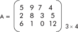
Now the matrix A of Figure 3.25 can be comfortably stored in the array called MAT_A[3][4] as shown in Figure 3.26.
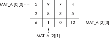
Let us consider a situation where it is desired that a value ‘5’ be added to all elements of the matrix ‘A’, stored in array called MAT_A. This operation can be done by picking the element MAT_A[0][0] (i.e., zeroth row and zeroth column) and adding the required value ‘5’ to its contents as shown below:
MAT_A[0][0] = MAT_A[0][0] + 5;
Now to complete the rest of the operations, there is a choice, i.e., either move along the zeroth row (MAT_A[0][1], MAT[0][2]…) and add ‘5’ to each visited element or to move along the zeroth col. (MAT_A[1][0], MAT[2][0]…) and add ‘5’ to each visited element. Once a row or column is over, we can move to the next row or column in the order and continue to travel in the same fashion.
Thus, a two-dimensional array can be travelled ‘row by row’ or ‘column by column’. The former method is called as row major order and the later as column major order.
An algorithm for row major order of travel of the array MAT_A is given below. This algorithm visits every element of the array MAT_A and adds the value ‘5’ to the contents of the visited element.
  Algorithm rowMajor()
  {
    Step
     1. for row = 0 to 2
     2. for col = 0 to 3
       MAT_A[row][col] = MAT_A[row][col] + 5;
     3. Stop
  }
In the above algorithm, nested loops have been used. The outer loop is employed to travel the rows and the inner to travel the columns within a given row.
Example 15: Given two matrices A[ ]m × r and B[ ]r × n , compute the product of two matrices such that:
C[ ]m × n = A [ ]m × r*B [ ]r × n
Solution: The multiplication of two matrices requires that a row of matrix A be multiplied to a column of matrix B to generate an element of matrix C as shown in Figure 3.27.
A close observation of the computation shown in Figure 3.27 gives the following relation for an element of matrix C:
C[I][J] = C[I][J] + A[I][K] × B[K][J] for k varying from 0 to r–1
We would use the above relation to compute the various elements of the matrix C. The required program is given below:
  /* This program multiplies two matrices A & B and stores the resultant matrix in C */
  #include <stdio.h>
  main()
  {
    int A[10][10], B[10][10], C[10][10];
    int i, j, k; /* The array indices */
    int m, n, r; /* Order of matrices */
    printf (“
 Enter the order of the matrices m, r, n:”);
    scanf (“%d %d %d”, &m,&r,&n);
    printf (“
 Enter The elements of Matrix A:”);
    for (i = 0; i < m; i++)
    for (j = 0; j < r; j++)
    {
      printf (“
 Enter an element : ”);
      scanf (“%d”, &A[i][j]);
    }
    printf (“
 Enter The elements of Matrix B :”);
    for (i = 0; i < r; i++)
    for (j = 0; j < n; j++)
    {
      printf (“
 Enter an element : ”);
      scanf (“%d”, &B[i][j]);
    }
                    /* Multiply the matrices */
    for (i = 0; i < m; i++)
    {
     for (j = 0; j < n; j++)
     {
      C[i][j] = 0;
      for (k = 0; k < r; k++)
      {
        C[i][j] = C[i][j] + A[i][k] * B[k][j];
      }
     }
    }
    printf (“
 The resultant matrix is ...
”);
    for (i = 0; i < m; i++)
    {
     for (j = 0; j < n; j++)
     {
       printf (“%d ”, C[i][j]);
     }
       printf (“
”);
    }
  }
Example 16: A nasty number is defined as a number which has at least two pairs of integer factors such that the difference of one pair equals to sum of the other pair. For instance, the factors of ‘6’ are 1, 2, 3, and 6.
Now the difference of factor pair (6, 1) is equal to sum of factor pair (2, 3), i.e., 6 – 1 = 2 + 3. Therefore, ‘6’ is a nasty number.
Choose appropriate data structure and write a program that displays all the nasty numbers present in a list of numbers.
Solution: The following data structures would be used to store the list of numbers and the list of factor-pair:
- A one-dimensional array called List to store the list of numbers.
- A two-dimensional array called pair_of_factors to store the list of pair-factors of a given number.
For example, the list of pair factors of ‘24’ would be stored as shown below:
| 1 | 24 |
| 2 | 12 |
| 3 | 8 |
| 4 | 6 |
Finally, using a nested loop, the difference of pair factors would be compared with the sum of all pair of factors for equality. The required program is given below:
  /* This program finds all the nasty numbers from a given list of integer numbers */
  #include <stdio.h>
  #include <math.h>
  main()
  {
    int LIST [20];
    int pair_of_factors[50][2];
    int i, j, k, size, num, diff, sum, count;

    printf (“
 Enter the size of the list : ”);
    scanf (“%d”, &size);

    printf (“
 Enter the list : ”);
    for (i = 0; i < size; i++)
    scanf (“%d”, &LIST[i]);

    for (i = 0; i<size; i++)
    {
     num = LIST[i];
     count = 0;
             /* Compute the factors */
     pair_of_factors[0][0] = 1;
     pair_of_factors[0][1] = num;
     for (j = 2 ; j <= sqrt(num); j++)
     {
       if (num % j == 0)
       {
        count++;
        pair_of_factors[count][0] = j;
        pair_of_factors[count][1] = num/j;
       }
     }
              /* Check for nastiness */
     for (j = 0; j <= count; j++)
     {
       diff = pair_of_factors[j][1] − pair_of_factors[j][0];
       for (k = 0; k < = count; k++)
       {
          sum = pair_of_factors[k][1] + pair_of_factors[k][0];
          if (diff == sum)
          {
            printf (“
 %d is a Nasty number”, num);
            break;
          }
        } /* End of k loop */
      } /* End of j loop */
    } /* End of i loop */
  } /* End of program */
3.4 REPRESENTATION OF ARRAYS IN PHYSICAL MEMORY
A programmer looks upon one-dimensional and two-dimensional arrays as ‘lists’ and ‘tables’ (or matrices), respectively. This is a logical view of the programmer about arrays as data structures, capable of storing lists or tables. However, at physical level, the main memory is RAM which is just a linear memory. The relationship between logical and physical views of arrays is shown in Figure 3.28.
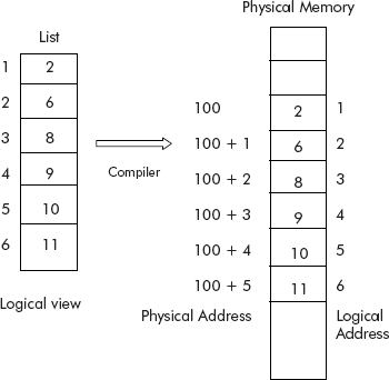
Thus, the compiler has to map the various locations of arrays to locations of the physical memory. In fact, for a given array index, the compiler computes its physical load time address of physical memory location. For example, List[5] would be loaded at physical address = 105, in the physical memory (see Figure 3.28).
Since physical memory is linear by construction, the address mapping is quite a simple exercise. The compiler needs to know only the starting address of the first element in the physical memory. The rest of the addresses can be generated by a trivial formula. A brief discussion on address computation is given in the subsequent sections.
3.4.1 Physical Address Computation of Elements of One-dimensional Arrays
Let us reconsider the array (LIST[N]) shown in Figure 3.28. The array called ‘LIST’ has six elements. It has been stored in physical memory at a stating address ‘100’. The address map is given below:
The address of 1st element = 100
2nd element = 100 + 1
3rd element = 100 + 2
_
_
6th element = 100 + 5
It is very easy to deduce from above address map that the equivalent physical address of an Ith element of array = 100 + (I – 1). The starting address of array at physical memory (i.e., 100) is called base address (Base) of the array. For example, the base address of array called LIST is ‘100’.
The formula for address of Ith location can be written as given below:
Eq. 3.5 is a simple case, i.e., it is assumed that every element of List would occupy only one location of the physical memory. However if an element of an array occupies ‘S’ number of memory locations, the Eq. 3.5 can be modified as as follows:
where
List: is the name of the array.
Base: is starting or base address of array.
I: is the index of the element.
S: is the number of locations occupied by an element of the array.
3.4.2 Physical Address Computation of Elements of Two-dimensional Arrays
Let us reconsider the two-dimensional array called TAB[2][3] as shown in Figure 3.29.
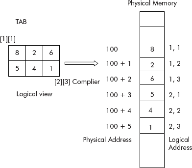
The array called ‘TAB’ has two rows and three columns. It has been stored in physical memory at a starting address ‘100’. The address map is given below:
The address of 1st row, 1st col = 100
1st row, 2nd col = 100 + 1
1st row, 3rd col = 100 + 2
_
_
2nd row, 3rd col = 100 + 5
We know that in two-dimensional array called TAB, for every row, there are three columns. Thus, for an element of Ith row the starting address becomes: Base + (I – 1)*3 and if the element in row is at Jth column, the complete address becomes:
To test the above row major order formula, let us calculate the address of element represented by TAB[2][1] with Base = 100.
Given: I = 2, J = 1, Base = 100. Putting these values in Eq. 3.7, we get
Address = 100 + (2 – 1)*3 + 1 – 1 = 100 + 3 + 0 = 103.
From Figure 3.29, we find that the address value is correct.
Now we can generalize the formula of Eq. 3.7 for an array of size [M][N] in the following form:
The formula given above is a simple case, i.e., it is assumed that every element of List would occupy only one location of the physical memory. However if an element of an array occupies ‘S’ number of memory locations, the row major order formula (3.8) can be modified as given below:
where
TAB: is the name of the array.
Base: is starting or base address of array.
I: is the row index of the element.
J: is the column index of the element.
N: is number of columns present in a row.
S: is the number of locations occupied by an element of the array.
Similarly, the formula for column major order is as follows:
where
TAB: is the name of the array.
Base: is starting or base address of array.
I: is the row index of the element.
J : is the column index of the element.
M: is number of rows present in a column.
S: is the number of locations occupied by an element of the array.
Example 17: TAB is a two-dimensional array with five rows and three columns. Each element occupies one memory location. If TAB[1][1] begins at address 500, find the location of TAB [4][2] for row major order of storage.
Solution
| Given base | = 500, I = 4, J = 2, M = 5, N = 3. Applying formula 3.9, we get: |
| Address | = Base + ((I – 1)*N + (J – 1))*S |
| = 500 + ((4 – 1)*3 + (2 – 1))*1 | |
| = 500 + (9 + 1) | |
| = 510. |
Example 18: MAT is a two-dimensional array with ten rows and five columns. Each element is stored in two memory locations. If MAT[1][1] begins at address 200, find the location of MAT [3][4] for row major order of storage.
Solution:
| Given base | = 200, I = 3, J = 4, M = 10, N = 5. Applying formula 3.9, we get: |
| Address | = Base + ((I – 1)*N + (J – 1))*S |
| = 200 + ((3 – 1)*5 + (4 – 1))*2 | |
| = 200 + (10 + 3)*2 | |
| = 226. |
Example 19: An array A[10][20] is stored in the memory with each element requiring two memory locations. If the base address of the array in the memory is 400, determine the location of array element A[8][3] when array is stored as column major order.
Solution:
| Given base | = 400, I = 8, J = 3, M = 10, N = 20. Applying formula 3.10, we get: |
| Address | = Base + ((J – 1)*M + (I – 1))*S |
| = 400 + ((3 – 1)*10 + (8 – 1))*2 | |
| = 400 + (20 + 7)*2 | |
| = 454. |
3.5 APPLICATIONS OF ARRAYS
The arrays are used data structures which are very widely in numerous applications. Some of the popular applications are:
3.5.1 Polynomial Representation and Operations
An expression of the form f(x) = an xn + an–1 xn–1 + an–2 xn–2 + ………..+ a0 is called a polynomial
where an ≠ 0.
an xn , an–1 xn–1,…. a1 x1 , a0 are called terms.
an, an-1 ,…. a1, a0 are called coefficient.
xn, xn–1 , xn–2 are called exponents,
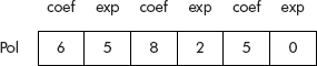
Now, a polynomial can be considered as a list comprising coefficients and exponents as shown below:
F(x) = {an, xn, an-1, xn–1,…. a1, x1 , a0 , x0}
For example, the polynomial 6x5 + 8x2 + 5 can be represented as the list shown below:
Polynomial = {6, 5, 8, 2, 5, 0}
The above list can be very easily implemented using a one-dimensional array, say Pol[] as shown in Figure 3.30 where every alternate location contains coefficient and exponent.
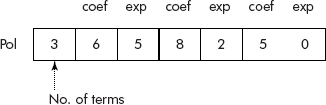
The above representation can be modified to incorporate number of terms present in a polynomial by reserving the zeroth location of the array for this purpose. The modified representation is shown in Figure 3.31.
It may be noted from the above discussion that a general polynomial can be represented in an array with descending order of its degree of terms. Therefore, the operations such as addition, multiplication, and division on polynomials can be easily carried out.
Example 20: Write a program that reads two polynomials pol1 and pol2, adds them and gives a third polynomial pol3 such that pol3 = pol1 + pol2.
Solution: A close look at the array representation of polynomials indicates, that two polynomials can be added by merging them using ‘algorithm merge()’ of Section 3.2.5.7. The only change would be that when the exponents from both the polynomials are same, then the coefficients of both the terms would be added.
The required program is given below:
  /* This program adds two polynomials pol1 and pol2 to give third polynomial called pol3. It merges the two polynomials with the help of Algorithm merge() with minor modifications * /
  #include <stdio.h>
  void readPol (int pol[], int terms);
  void dispPol (int pol[]);
  void main()
  {
    int pol1[11];
    int pol2[11];
    int pol3[21];
    int i, j, k;
    int terms;
    int m, n; /* size of polynomials */

    printf (“
 Enter the number of terms in Pol1”);
    scanf (“%d”, &terms);
    m = terms*2 + 1;

    readPol(pol1,terms);

    printf (“
 Enter the number of terms in Pol2”);
    scanf (“%d”, &terms);
    n = terms*2 + 1;

    readPol(pol2,terms);

             /* Add the polynomials by merging their terms */
    i = j = k = 2;

    while (i < m && j < n)
    {
      if (pol1[i] > pol2[j])
      {
       pol3[k] = pol1[i];
       pol3[k − 1] = pol1[i − 1];
       i = i + 2;
       k = k + 2;
      }
      else
      if (pol2[j] > pol1[i])
      {
        pol3[k] = pol2[j];
        pol3[k − 1] = pol2[j − 1];
        j = j + 2;
        k = k + 2;
      }
      else
      {
        pol3[k − 1] = pol1[i − 1] + pol2[j − 1];
        pol3[k] = pol1[i];
        I=i+2;
        j= j+2;
        k= k+2;
      }
    }
               /* copy the remaining Pol1 */
    while (i < m)
    {
      pol3[k] = pol1[i];
      pol3[k − 1] = pol1[i − 1];
      i = i + 2;
      k = k + 2;
    }
                 /* copy the remaining Pol2 */
    while (j < n)
    {
      pol3[k] = pol2[j];
      pol3[k − 1] = pol2[j − 1];
      j = j + 2;
      k = k + 2;
    }
    pol3[0] = (k − 1)/2;
                       /* Display the final polynomial */
    printf (“
 Final Pol =”);
    dispPol(pol3);
    printf (“”);
   }
   void readPol(int pol[], int terms)
   {
     int i;
     pol[0] = terms;
     i = 1;
     printf (“
 Enter the terms (coef exp) in decreasing order of degree”);

     while (terms > 0)
     {
       scanf (“%d %d”, &pol[i], &pol[i+1]);
       i = i + 2;
       terms−−;
     }
   }
   void dispPol(int pol[])
   {
    int size;
    int i;
    size = pol[0]*2 + 1;
    printf (“
”);
    for (i = 1; i < size; i + = 2)
    {
      printf (“%d*x^%d+”, pol[i], pol[i + 1]);
    }
  }
We can also choose other data structures to represent polynomials. For instance, a term can be represented by ‘struct’ construct of ‘C’ as shown below:
  struct term
   {
     int coef;
     int exp;
   };
and the polynomial called ‘pol’ of ten terms can be represented by an array of structures of type ‘term’ as shown below:
struct term pol1[10];
Now the algorithm merge() can be applied to add two such polynomials with above chosen data structures. It is left as an exercise for the readers to write that program.
3.5.2 Sparse Matrix Representation
A matrix is called sparse when it contains a large number of zero entries. Consider the matrix given in Figure 3.32.
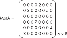
It may be noted that the matrix MatA of order 6 × 8 has 54 zero entries out of total 64 entries. Thus, it has enough number of zero entries that prompts us to look for an alternate representation that could save the memory space occupied by zero entries. A popular representation of a sparse matrix is given below.
A sparse matrix can be very easily represented by a list of ordered pairs. An ordered pair has the following format
                      (Row, Col, E)
    Where Row: is the row number
           Col: is the column number
             E: is the non zero entry at the given row and col.
Lets us now apply the above representation to MatA to obtain the list of ordered pairs as given below:
                0, 4, 2
                1, 1, 3
                1, 6, 5
                3, 3, 7
                4, 6, 4
                5, 0, 8
The above representation is also called a condensed matrix. It is using comparatively very less space which will become even prominent for large matrices, say of the order of 500 × 500 or more.
The proposed list of ordered pairs can be modeled as a two dimensional matrix of order of n + 1 × 3. Where n is the number of nonzero elements present in a sparse matrix. However, the 0th ordered pair can be suitably used to store the order of the sparse matrix and the number of nonzero elements present in the matrix as shown in Figure 3.33.
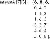
Example 21: Write a program that reads a sparse matrix of order m*n and stores it into the condensed representation as discussed above i.e. a two dimensional array of size n+1 * 3. Where n is number of non zero elements. Print the contents of the condensed matrix.
Solution: The required program is given below:
  /* This program reads a sparse matrix of order m*n and stores it into a condensed matrix format */
  # include <stdio.h>
  # include <conio.h>
  main()
  {
    int matA[7][3];
    int i,j,k;
    int m,n, element;
    clrscr();
    printf (“
 Enter the order (m,n) of the sparse matrix”);
    scanf (“%d %d”, &m,&n);
    matA[0][0] = m; /* no. of rows */
    matA[0][1] = n; /* no. of cols */
    k=1; /* point to 1st position of sparse mat */
    printf (“
 Enter the elements of the matrix in row major order”);
        for (i=0; i<m; i++)
      for (j=0; j < n; j++)
      {
        scanf (“%d”, &element);
        if (element != 0)
      {           /* store non zero element into condensed matrix */
        matA[k][0] = i;
        matA[k][1] = j;
        matA[k][2] = element;
        k++;
      }
     }
     matA[0][2] = k-1;               /* record no. of non zero elements */
    printf (“
 The condensed matrix is...”);
    for (i=1;i <k; i++)
     printf (“
 %d %d %d”, matA[i][0], matA[i][1],matA[i][2]);
  }
Note: No space has been provided for the sparse matrix. The elements have been read one by one and the nonzero elements have been stored into the condensed matrix.
A sample run of the program is given below:
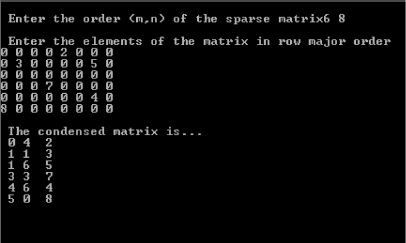
3.5.2.1 Sparse Matrix Addition
Two sparse matrices can be added in the same way as the polynomials were added in previous section. Consider the three sparse matrices Mat1, Mat2, and Mat3 given in Figure 3.34.
where Mat3 = Mat1 + Mat2
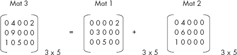
The equivalent condensed form of Mat1, Mat2, Mat3 is given in Figure 3.35.
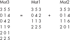
It may be noted that the final matrix Mat3, is nothing but a merger of two ordered lists Mat1 and Mat2 in a manner similar to polynomials. The ‘algorithm merge()’ of section 3.2.5.7 can be very easily applied. The only change would be that when the row number and column number from both the condensed matrices are same then the elements of both the matrices would be added. For example, merger of (1 1 3) and (1 1 6) would result into the element (1 1 9).
Example 22: Write a program that reads two sparse matrices Mat1 and Mat2 of order m*n, and represents them in condensed form. The condensed matrices are added to give a third condensed matrix called Mat3. It prints Mat3 in row major order.
Solution: We would use following three functions:
readMat(): It reads a sparse matrix and stores it into a condensed form
addsparsMat(): It takes two condensed matrices and adds them into a third condensed matrix
printMat(): It prints a condensed matrix
The required program is given below:
  /* This program adds two sparse matrices of order m*n */
  # include <stdio.h>
  # include <conio.h>
  void readMat (int matA[][], int m, int n);
  void printMat(int matA[][]);
  void addsparsMat (int mat1[][], int mat2[][], int mat3[][]);
  void main()
  {
    int mat1[10][3], mat2[10][3], mat3[20][3];
    int m,n;
    clrscr();
    printf (“
 Enter the order of the sparse mat1 : m, n”);
    scanf (“%d %d”, &m, &n);
    readMat(mat1,m,n);
    printMat(mat1);
    printf (“
 Enter the order of the sparse mat2 : m, n”);
    scanf (“%d %d”, &m, &n);
    readMat(mat2,m,n);
    printMat(mat2);
    addsparsMat (mat1,mat2,mat3);
    printf (“
 The final condensed Matrix”);
    printMat(mat3);
  }
  void readMat (int matA[10][3], int m, int n)
  {
    int i,j,k;
    int element;
    matA[0][0] = m;                      /* no. of rows */
    matA[0][1] = n;                      /* no. of cols */
    k=1;                                 /* point to 1st position of sparse mat */
    printf (“
 Enter the elements of the matrix in row major order”);
       for (i=0; i<m; i++)
      for (j=0; j < n; j++)
      {
       scanf (“%d”, &element);
       if (element != 0)
       {
        matA[k][0] = i;
        matA[k][1] = j;
        matA[k][2] = element;
        k++;
       }
     }
    matA[0][2] = k-1;          /* record no. of non zero elements */
  }
  void printMat(int matA[10][3])
  {
    int i, size;
    size = matA[0][2];
    for (i=0 ; i<= size; i++)
      printf (“
 %d %d %d”, matA[i][0], matA[i][1],matA[i][2]);
  }
  void addsparsMat (int mat1[10][3], int mat2[10][3], int mat3[20][3])
  {
    int i,j,k;
    int s1,s2; /* No. of elements in mat1 and mat2 */
    s1 = mat1[0][2];
    s2 = mat2[0][2];
    i=j=k=0;
    while ( i <= s1 && j <= s2)
    {
    if (mat1[i][0] < mat2[j][0]) /* row of mat1 < mat2 */
    {
      mat3[k][0] = mat1[i][0];
      mat3[k][1] = mat1[i][1];
      mat3[k][2] = mat1[i][2];
      k++; i++;
    }
    else
     if (mat1[i][0] > mat2[j][0]) /* row of mat1 > mat2 */
     {
        mat3[k][0] = mat2[j][0];
        mat3[k][1] = mat2[j][1];
        mat3[k][2] = mat2[j][2];
        k++; j++;
     }
     else
     {                                    /* row of mat1 = mat2 */
       if (mat1[i][1] < mat2[j][1]) /* col of mat1 < mat2 */
       {
         mat3[k][0] = mat1[i][0];
         mat3[k][1] = mat1[i][1];
         mat3[k][2] = mat1[i][2];
         k++; i++;
       }
       else
       if (mat1[i][1] > mat2[j][1]) /* col of mat1 > mat2 */
       {
         mat3[k][0] = mat2[j][0];
         mat3[k][1] = mat2[j][1];
         mat3[k][2] = mat2[j][2];
         k++; j++;
       }
       else
       {       /* col of mat1 = mat2 */
         mat3[k][0] = mat2[i][0];
         mat3[k][1] = mat2[i][1];
         mat3[k][2] = mat1[i][2] + mat2[j][2];
         k++;i++;j++;
       }
     }
   }
   while (i <= s1) /* copy rest of the elements of mat1 */
   {
     mat3[k][0] = mat1[i][0];
     mat3[k][1] = mat1[i][1];
     mat3[k][2] = mat1[i][2];
     k++; i++;
   }
   while (j <= s2) /* copy rest of the elements of mat2 */
   {
     mat3[k][0] = mat2[j][0];
     mat3[k][1] = mat2[j][1];
     mat3[k][2] = mat1[j][2];
     k++;j++;
   }
   mat3[0][2] =k-1;
  }
A sample output of the program is given below:
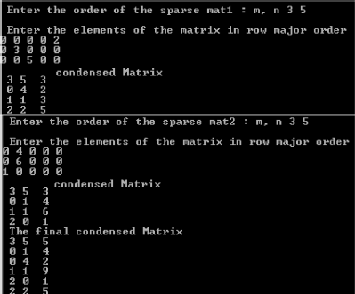
3.5.2.2 Sparse Matrix Transpose
The transpose of a matrix of order m * n is defined as a matrix n *m that is formed by interchanging the rows and columns of the matrix. In fact, the transpose of the matrix is obtained by exchanging the element at (i, j) th position in the matrix t with the element at (j, i)th place as shown in Figure 3.36.
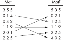
It may be noted that the number of rows and number of columns have also been exchanged.
Example 23: Write a program that produces a transpose of a given sparse matrix of order m*n.
Solution: The required program is given below
  /* This program produces a Transpose of a sparse matrix */
  # include <stdio.h>
  # include <conio.h>
  void readMat (int matA[][], int m, int n);
  void printMat(int matA[][]);
  void transMat (int mat[][], int trans[][]);
  void main()
  {
    int mat[10][3], trans[10][3];
    int m,n;
    clrscr();
    printf (“
 Enter the order of the sparse mat : m, n”);
    scanf (“%d %d”, &m, &n);
    readMat(mat,m,n);
    printMat(mat);
    transMat (mat,trans);
    printf (“
 The transposed condensed Matrix”);
    printMat(trans);
  }
  void readMat (int matA[10][3], int m, int n)
  {
    int i,j,k;
    int element;
    matA[0][0] = m; /* no. of rows */
    matA[0][1] = n; /* no. of cols */
    k=1; /* point to 1st position of sparse mat */
    printf (“
 Enter the elements of the matrix in row major order”);
        for (i=0; i<m; i++)
       for (j=0; j < n; j++)
       {
         scanf (“%d”, &element);
         if (element != 0)
         {
           matA[k][0] = i;
           matA[k][1] = j;
           matA[k][2] = element;
           k++;
         }
       }
    matA[0][2] = k-1; /* record no. of non zero elements */
   }
   void printMat(int matA[10][3])
   {
     int i, size;
     size = matA[0][2];
     for (i=0 ; i<= size; i++)
     printf (“
 %d %d %d”, matA[i][0], matA[i][1],matA[i][2]);
   }
   void transMat (int mat[10][3], int trans[10][3])
   {
     int i, j, small, size,pos,temp;
     size = mat[0][2];
     trans[0][0] = mat[0][1];
     trans[0][1] = mat[0][0];
     trans[0][2] = mat[0][2];
     for (i=1; i<=size; i++)
     {
       trans[i][0] = mat[i][0];
       trans[i][1] = mat[i][1];
       trans[i][2] = mat[i][2];
     }
     for (i=1; i < size; i++)
     {
       small = trans[i][1]; pos =i;
       for (j = i+1; j <=size; j++)
       {
        if (small > trans[j][1])
        {
          small = trans[j][1];
          pos = j;
        }
       else
       if (small == trans[j][1] && trans[i][0] > trans[j][0])
       {
         small = trans[j][1];
         pos = j;
       }
     }
       temp =trans[i][0];trans[i][0] = trans[pos][0];trans[pos][0] =temp;
       temp =trans[i][1];trans[i][1] = trans[pos][1];trans[pos][1] =temp;
       temp =trans[i][2];trans[i][2] = trans[pos][2];trans[pos][2] =temp;
       temp =trans[i][0];trans[i][0] = trans[i][1]; trans[i][1] = temp;
     }
  }
A sample output is given below:
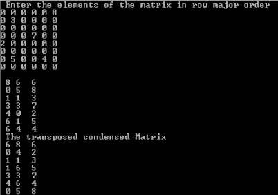
EXERCISES
- Define the terms: array, subscript, subscripted variables and strings.
- Write suitable array declaration for the following:
- 100 items of integer type.
- A string of 25 characters.
- A matrix of order 5 × 4.
- Can an array be initialized? If yes, how?
- What is the purpose of initializing an array?
- Can array be initialized at the time of declaration?
- How can a string be stored in an array?
- Write a program that finds the largest and smallest elements in an array.
- Write a program that removes duplicate from a list.
- Write a program that removes an element from an array.
- Write a program that searches an array SOME of float type for a value less that x. The program should give appropriate message depending upon the outcome of the search.
- Write a program which searches an ordered array SAL of integer type for a value X.
- Write a program that gives the sum of positive elements of an array LIST of integer type.
- Write a program that reads two matrices A and B of order m × n and compute the following:
C = A + B
- What happens to an array if it is assigned with less number of elements at the time of initialization?
- Write a program that computes the sum of diagonal elements of a square matrix.
- Write a program that takes a sparse matrix A and finds its transpose AT and displays it.
- Let A be an N × N square matrix array. Write algorithms for the following:
- Find the number of non-zero elements in A.
- Find the product of the diagonal elements (a11, a22, a33,……ann).
- Find out the complexity of binary search. Compare its time complexity with linear search.
- What is meant by sorting? What are the types of sorting?
- What is the difference between bubble sort and selection sort?
- What is meant by quick sort? What are the advantages/disadvantages of quick sort over merge sort?
- Explain how the selection of pivot plays major role in efficiency of quick sort algorithm and determine the complexity of the quick sort.
- Trace the steps of insertion sort for the list of numbers: 12, 19, 33, 26, 29, 35, 22. Compute the total number of comparisons made.
- What is shell sort? Define the worst case analysis of shell sort.
- What is merge sort? Write algorithm for merge sort and derive its run time complexity.
- How the two-dimensional arrays are represented in memory? Also, obtain the formula for calculating the address of any element stored in the array, in column major order.
- Write a program that sorts a given list of numbers using bubble sort.
- Write a program that sorts a given list of numbers using selection sort.
- Derive the time complexity of selection sort.
- Derive the time complexity of insertion sort.
- Write a program that sorts a given list of numbers using quick sort.
- Write a program that sorts a given list of numbers using merge sort.