
Chapter 32. Approximate Aggregations
Life is easy if all your data fits on a single machine. Classic algorithms taught in CS201 will be sufficient for all your needs. But if all your data fits on a single machine, there would be no need for distributed software like Elasticsearch at all. But once you start distributing data, algorithm selection needs to be made carefully.
Some algorithms are amenable to distributed execution. All of the aggregations
discussed thus far execute in a single pass and give exact results. These types
of algorithms are often referred to as embarrassingly parallel,
because they parallelize to multiple machines with little effort. When
performing a max metric, for example, the underlying algorithm is very simple:
-
Broadcast the request to all shards.
-
Look at the
pricefield for each document. Ifprice > current_max, replacecurrent_maxwithprice. -
Return the maximum price from all shards to the coordinating node.
-
Find the maximum price returned from all shards. This is the true maximum.
The algorithm scales linearly with machines because the algorithm requires no coordination (the machines don’t need to discuss intermediate results), and the memory footprint is very small (a single integer representing the maximum).
Not all algorithms are as simple as taking the maximum value, unfortunately. More complex operations require algorithms that make conscious trade-offs in performance and memory utilization. There is a triangle of factors at play: big data, exactness, and real-time latency.
You get to choose two from this triangle:
- Exact + real time
-
Your data fits in the RAM of a single machine. The world is your oyster; use any algorithm you want. Results will be 100% accurate and relatively fast.
- Big data + exact
-
A classic Hadoop installation. Can handle petabytes of data and give you exact answers—but it may take a week to give you that answer.
- Big data + real time
-
Approximate algorithms that give you accurate, but not exact, results.
Elasticsearch currently supports two approximate algorithms (cardinality and
percentiles). These will give you accurate results, but not 100% exact.
In exchange for a little bit of estimation error, these algorithms give you
fast execution and a small memory footprint.
For most domains, highly accurate results that return in real time across all your data is more important than 100% exactness. At first blush, this may be an alien concept to you. “We need exact answers!” you may yell. But consider the implications of a 0.5% error:
-
The true 99th percentile of latency for your website is 132ms.
-
An approximation with 0.5% error will be within +/- 0.66ms of 132ms.
-
The approximation returns in milliseconds, while the “true” answer may take seconds, or be impossible.
For simply checking on your website’s latency, do you care if the approximate answer is 132.66ms instead of 132ms? Certainly, not all domains can tolerate approximations—but the vast majority will have no problem. Accepting an approximate answer is more often a cultural hurdle rather than a business or technical imperative.
Finding Distinct Counts
The first approximate aggregation provided by Elasticsearch is the cardinality
metric. This provides the cardinality of a field, also called a distinct or
unique count. You may be familiar with the SQL version:
SELECTDISTINCT(color)FROMcars
Distinct counts are a common operation, and answer many fundamental business questions:
-
How many unique visitors have come to my website?
-
How many unique cars have we sold?
-
How many distinct users purchased a product each month?
We can use the cardinality metric to determine the number of car colors being
sold at our dealership:
GET/cars/transactions/_search?search_type=count{"aggs":{"distinct_colors":{"cardinality":{"field":"color"}}}}
This returns a minimal response showing that we have sold three different-colored cars:
..."aggregations":{"distinct_colors":{"value":3}}...
We can make our example more useful: how many colors were sold each month? For
that metric, we just nest the cardinality metric under a date_histogram:
GET/cars/transactions/_search?search_type=count{"aggs":{"months":{"date_histogram":{"field":"sold","interval":"month"},"aggs":{"distinct_colors":{"cardinality":{"field":"color"}}}}}}
Understanding the Trade-offs
As mentioned at the top of this chapter, the cardinality metric is an approximate
algorithm. It is based on the HyperLogLog++ (HLL) algorithm. HLL works by
hashing your input and using the bits from the hash to make probabilistic estimations
on the cardinality.
You don’t need to understand the technical details (although if you’re interested, the paper is a great read!), but you should be aware of the properties of the algorithm:
-
Configurable precision, which controls memory usage (more precise == more memory).
-
Excellent accuracy on low-cardinality sets.
-
Fixed memory usage. Whether there are thousands or billions of unique values, memory usage depends on only the configured precision.
To configure the precision, you must specify the precision_threshold parameter.
This threshold defines the point under which cardinalities are expected to be very
close to accurate. Consider this example:
GET/cars/transactions/_search?search_type=count{"aggs":{"distinct_colors":{"cardinality":{"field":"color","precision_threshold":100
}}}}
precision_thresholdaccepts a number from 0–40,000. Larger values are treated as equivalent to 40,000.
This example will ensure that fields with 100 or fewer distinct values will be extremely accurate. Although not guaranteed by the algorithm, if a cardinality is under the threshold, it is almost always 100% accurate. Cardinalities above this will begin to trade accuracy for memory savings, and a little error will creep into the metric.
For a given threshold, the HLL data-structure will use about
precision_threshold * 8 bytes of memory. So you must balance how much memory
you are willing to sacrifice for additional accuracy.
Practically speaking, a threshold of 100 maintains an error under 5% even when
counting millions of unique values.
Optimizing for Speed
If you want a distinct count, you usually want to query your entire dataset (or nearly all of it). Any operation on all your data needs to execute quickly, for obvious reasons. HyperLogLog is very fast already—it simply hashes your data and does some bit-twiddling.
But if speed is important to you, we can optimize it a little bit further. Since HLL simply needs the hash of the field, we can precompute that hash at index time. When the query executes, we can skip the hash computation and load the value directly out of fielddata.
Note
Precomputing hashes is useful only on very large and/or high-cardinality fields. Calculating the hash on these fields is non-negligible at query time.
However, numeric fields hash very quickly, and storing the original numeric often requires the same (or less) memory. This is also true on low-cardinality string fields; there are internal optimizations that guarantee that hashes are calculated only once per unique value.
Basically, precomputing hashes is not guaranteed to make all fields faster — only those that have high cardinality and/or large strings. And remember, precomputing simply shifts the cost to index time. You still pay the price; you just choose when to pay it.
To do this, we need to add a new multifield to our data. We’ll delete our index, add a new mapping that includes the hashed field, and then reindex:
DELETE/cars/PUT/cars/{"mappings":{"color":{"type":"string","fields":{"hash":{"type":"murmur3"}}}}}POST/cars/transactions/_bulk{"index":{}}{"price":10000,"color":"red","make":"honda","sold":"2014-10-28"}{"index":{}}{"price":20000,"color":"red","make":"honda","sold":"2014-11-05"}{"index":{}}{"price":30000,"color":"green","make":"ford","sold":"2014-05-18"}{"index":{}}{"price":15000,"color":"blue","make":"toyota","sold":"2014-07-02"}{"index":{}}{"price":12000,"color":"green","make":"toyota","sold":"2014-08-19"}{"index":{}}{"price":20000,"color":"red","make":"honda","sold":"2014-11-05"}{"index":{}}{"price":80000,"color":"red","make":"bmw","sold":"2014-01-01"}{"index":{}}{"price":25000,"color":"blue","make":"ford","sold":"2014-02-12"}
This multifield is of type
murmur3, which is a hashing function.
Now when we run an aggregation, we use the color.hash field instead of the
color field:
GET/cars/transactions/_search?search_type=count{"aggs":{"distinct_colors":{"cardinality":{"field":"color.hash"}}}}
Notice that we specify the hashed multifield, rather than the original.
Now the cardinality metric will load the values (the precomputed hashes)
from "color.hash" and use those in place of dynamically hashing the original
value.
The savings per document is small, but if hashing each field adds 10 nanoseconds and your aggregation touches 100 million documents, that adds 1 second per
query. If you find yourself using cardinality across many documents,
perform some profiling to see if precomputing hashes makes sense for your
deployment.
Calculating Percentiles
The other approximate metric offered by Elasticsearch is the percentiles metric.
Percentiles show the point at which a certain percentage of observed values occur.
For example, the 95th percentile is the value that is greater than 95% of the
data.
Percentiles are often used to find outliers. In (statistically) normal distributions, the 0.13th and 99.87th percentiles represent three standard deviations from the mean. Any data that falls outside three standard deviations is often considered an anomaly because it is so different from the average value.
To be more concrete, imagine that you are running a large website and it is your job to guarantee fast response times to visitors. You must therefore monitor your website latency to determine whether you are meeting your goal.
A common metric to use in this scenario is the average latency. But this is a poor choice (despite being common), because averages can easily hide outliers. A median metric also suffers the same problem. You could try a maximum, but this metric is easily skewed by just a single outlier.
This graph in Figure 32-1 visualizes the problem. If you rely on simple metrics like mean or median, you might see a graph that looks like Figure 32-1.
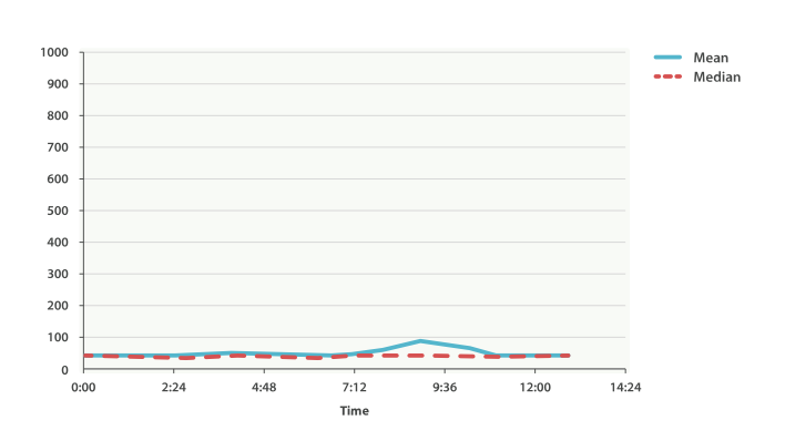
Figure 32-1. Average request latency over time
Everything looks fine. There is a slight bump, but nothing to be concerned about. But if we load up the 99th percentile (the value that accounts for the slowest 1% of latencies), we see an entirely different story, as shown in Figure 32-2.
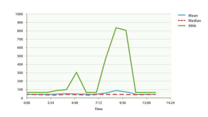
Figure 32-2. Average request latency with 99th percentile over time
Whoa! At 9:30 a.m., the mean is only 75ms. As a system administrator, you wouldn’t look at this value twice. Everything normal! But the 99th percentile is telling you that 1% of your customers are seeing latency in excess of 850ms—a very different story. There is also a smaller spike at 4:48 a.m. that wasn’t even noticeable in the mean/median.
This is just one use-case for a percentile. Percentiles can also be used to quickly eyeball the distribution of data, check for skew or bimodalities, and more.
Percentile Metric
Let’s load a new dataset (the car data isn’t going to work well for percentiles). We are going to index a bunch of website latencies and run a few percentiles over it:
POST/website/logs/_bulk{"index":{}}{"latency":100,"zone":"US","timestamp":"2014-10-28"}{"index":{}}{"latency":80,"zone":"US","timestamp":"2014-10-29"}{"index":{}}{"latency":99,"zone":"US","timestamp":"2014-10-29"}{"index":{}}{"latency":102,"zone":"US","timestamp":"2014-10-28"}{"index":{}}{"latency":75,"zone":"US","timestamp":"2014-10-28"}{"index":{}}{"latency":82,"zone":"US","timestamp":"2014-10-29"}{"index":{}}{"latency":100,"zone":"EU","timestamp":"2014-10-28"}{"index":{}}{"latency":280,"zone":"EU","timestamp":"2014-10-29"}{"index":{}}{"latency":155,"zone":"EU","timestamp":"2014-10-29"}{"index":{}}{"latency":623,"zone":"EU","timestamp":"2014-10-28"}{"index":{}}{"latency":380,"zone":"EU","timestamp":"2014-10-28"}{"index":{}}{"latency":319,"zone":"EU","timestamp":"2014-10-29"}
This data contains three values: a latency, a data center zone, and a date
timestamp. Let’s run percentiles over the whole dataset to get a feel for
the distribution:
GET/website/logs/_search?search_type=count{"aggs":{"load_times":{"percentiles":{"field":"latency"}},"avg_load_time":{"avg":{"field":"latency"
}}}}
The
percentilesmetric is applied to thelatencyfield.For comparison, we also execute an
avgmetric on the same field.
By default, the percentiles metric will return an array of predefined percentiles:
[1, 5, 25, 50, 75, 95, 99]. These represent common percentiles that people are
interested in—the extreme percentiles at either end of the spectrum, and a
few in the middle. In the response, we see that the fastest latency is around 75ms,
while the slowest is almost 600ms. In contrast, the average is sitting near
200ms, which is much less informative:
..."aggregations":{"load_times":{"values":{"1.0":75.55,"5.0":77.75,"25.0":94.75,"50.0":101,"75.0":289.75,"95.0":489.34999999999985,"99.0":596.2700000000002}},"avg_load_time":{"value":199.58333333333334}}
So there is clearly a wide distribution in latencies. Let’s see whether it is correlated to the geographic zone of the data center:
GET/website/logs/_search?search_type=count{"aggs":{"zones":{"terms":{"field":"zone"},"aggs":{"load_times":{"percentiles":{"field":"latency","percents":[50,95.0,99.0]
}},"load_avg":{"avg":{"field":"latency"}}}}}}
First we separate our latencies into buckets, depending on their zone.
Then we calculate the percentiles per zone.
The
percentsparameter accepts an array of percentiles that we want returned, since we are interested in only slow latencies.
From the response, we can see the EU zone is much slower than the US zone. On the US side, the 50th percentile is very close to the 99th percentile—and both are close to the average.
In contrast, the EU zone has a large difference between the 50th and 99th percentile. It is now obvious that the EU zone is dragging down the latency statistics, and we know that 50% of the EU zone is seeing 300ms+ latencies.
..."aggregations":{"zones":{"buckets":[{"key":"eu","doc_count":6,"load_times":{"values":{"50.0":299.5,"95.0":562.25,"99.0":610.85}},"load_avg":{"value":309.5}},{"key":"us","doc_count":6,"load_times":{"values":{"50.0":90.5,"95.0":101.5,"99.0":101.9}},"load_avg":{"value":89.66666666666667}}]}}...
Percentile Ranks
There is another, closely related metric called percentile_ranks. The
percentiles metric tells you the lowest value below which a given percentage of documents fall. For instance, if the 50th percentile is 119ms, then 50% of documents have values of no more than 119ms. The percentile_ranks tells you which percentile a specific value belongs to. The percentile_ranks of 119ms is the 50th percentile. It is basically a two-way relationship. For example:
-
The 50th percentile is 119ms.
-
The 119ms percentile rank is the 50th percentile.
So imagine that our website must maintain an SLA of 210ms response times or less. And, just for fun, your boss has threatened to fire you if response times creep over 800ms. Understandably, you would like to know what percentage of requests are actually meeting that SLA (and hopefully at least under 800ms!).
For this, you can apply the percentile_ranks metric instead of percentiles:
GET/website/logs/_search?search_type=count{"aggs":{"zones":{"terms":{"field":"zone"},"aggs":{"load_times":{"percentile_ranks":{"field":"latency","values":[210,800]}}}}}}
The
percentile_ranksmetric accepts an array of values that you want ranks for.
After running this aggregation, we get two values back:
"aggregations":{"zones":{"buckets":[{"key":"eu","doc_count":6,"load_times":{"values":{"210.0":31.944444444444443,"800.0":100}}},{"key":"us","doc_count":6,"load_times":{"values":{"210.0":100,"800.0":100}}}]}}
This tells us three important things:
-
In the EU zone, the percentile rank for 210ms is 31.94%.
-
In the US zone, the percentile rank for 210ms is 100%.
-
In both EU and US, the percentile rank for 800ms is 100%.
In plain english, this means that the EU zone is meeting the SLA only 32% of the time, while the US zone is always meeting the SLA. But luckily for you, both zones are under 800ms, so you won’t be fired (yet!).
The percentile_ranks metric provides the same information as percentiles, but
presented in a different format that may be more convenient if you are interested in specific value(s).
Understanding the Trade-offs
Like cardinality, calculating percentiles requires an approximate algorithm. The naive implementation would maintain a sorted list of all values—but this clearly is not possible when you have billions of values distributed across dozens of nodes.
Instead, percentiles uses an algorithm called TDigest (introduced by Ted Dunning
in Computing Extremely Accurate Quantiles Using T-Digests). As with HyperLogLog, it isn’t
necessary to understand the full technical details, but it is good to know
the properties of the algorithm:
-
Percentile accuracy is proportional to how extreme the percentile is. This means that percentiles such as the 1st or 99th are more accurate than the 50th. This is just a property of how the data structure works, but it happens to be a nice property, because most people care about extreme percentiles.
-
For small sets of values, percentiles are highly accurate. If the dataset is small enough, the percentiles may be 100% exact.
-
As the quantity of values in a bucket grows, the algorithm begins to approximate the percentiles. It is effectively trading accuracy for memory savings. The exact level of inaccuracy is difficult to generalize, since it depends on your data distribution and volume of data being aggregated.
Similar to cardinality, you can control the memory-to-accuracy ratio by changing
a parameter: compression.
The TDigest algorithm uses nodes to approximate percentiles: the more nodes available, the higher the accuracy (and the larger the memory footprint)
proportional to the volume of data. The compression parameter limits the maximum
number of nodes to 20 * compression.
Therefore, by increasing the compression value, you can increase the accuracy of
your percentiles at the cost of more memory. Larger compression values also
make the algorithm slower since the underlying tree data structure grows in size, resulting in more expensive operations. The default compression value is 100.
A node uses roughly 32 bytes of memory, so in a worst-case scenario (for example, a large amount of data that arrives sorted and in order), the default settings will produce a TDigest roughly 64KB in size. In practice, data tends to be more random, and the TDigest will use less memory.