CHAPTER 2
Numerical Algorithms
Numerical Algorithms calculate numbers. They perform such tasks as randomizing values, breaking numbers into their prime factors, finding greatest common divisors, and computing geometric areas.
All these algorithms are useful occasionally, but they also demonstrate useful algorithmic techniques such as adaptive algorithms, Monte Carlo simulation, and using tables to store intermediate results.
Randomizing Data
Randomization plays an important role in many applications. It lets a program simulate random processes, test algorithms to see how they behave with random inputs, and search for solutions to difficult problems. Monte Carlo integration, which is described in the later section “Performing Numerical Integration,” uses randomly selected points to estimate the size of a complex geometric area.
The first step in any randomized algorithm is generating random numbers.
Generating Random Values
Even though many programmers talk about “random” number generators, any algorithm used by a computer to produce numbers is not truly random. If you knew the details of the algorithm and its internal state, you could correctly predict the “random” numbers it generates.
To get truly unpredictable randomness, you need to use a source other than a computer program. For example, you could use a radiation detector that measures particles coming out of a radioactive sample to generate random numbers. Because no one can predict exactly when the particles will emerge, this is truly random.
Other possible sources of true randomness include dice rolls, analyzing static in radio waves, and studying Brownian motion. Random.org measures atmospheric noise to generate random numbers. (You can go to http://www.random.org to get true random numbers.)
Unfortunately, because these sorts of true random-number generators (TRNG) are relatively complicated and slow, most applications use a faster pseudorandom number generator (PRNG) instead. For many applications, if the numbers are in some sense “random enough,” a program can still make use of them and get good results.
Generating Values
One simple and common method of creating pseudorandom numbers is a linear congruential generator, which uses the following relationship to generate numbers:
![]()
A, B, and M are constants.
The value of X0 initializes the generator so that different values for X0 produce different sequences of numbers. A value that is used to initialize the pseudorandom number generator, such as X0 in this case, is called the seed.
Because all the values in the number sequence are taken modulo M, after at most M numbers the generator produces a number it produced before, and the sequence of numbers repeats from that point.
As a very small example, suppose A = 7, B = 5, and M = 11. If you start with X0 = 0, the previous equation gives you the following sequence of numbers:
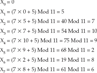
Because X10 = X0 = 0, the sequence repeats.
The values 0, 5, 7, 10, 9, 2, 8, 6, 3, 4 look fairly random. But now that you know the method that the program uses to generate the numbers, if someone tells you the method's current number, you can correctly predict those that follow.
Some PRNG algorithms use multiple linear congruential generators with different constants and then select from among the values generated at each step to make the numbers seem more random and to increase the sequence's repeat period. That can make programs produce more random-seeming results, but those methods are still not truly random.
NOTE Most programming languages have built-in PRNG methods that you can use instead of writing your own. Those methods generally are reasonably fast and produce very long sequences of numbers before they repeat, so for most programs you can simply use them instead of writing your own.
One feature of PRNGs that is sometimes an advantage is that you can use a particular seed value to generate the same sequence of “random” values repeatedly. That may seem like a disadvantage, because it means that the numbers are more predictable, but being able to use the same numbers repeatedly can make some programs much easier to debug.
Being able to repeat sequences of numbers also lets some applications store complex data in a very compact form. For example, suppose a program needs to make an object perform a long and complicated pseudorandom walk on a map. The program could generate the walk and save all its coordinates so that it can redraw the route later. Alternatively, it could just save a seed value. Then, whenever it needs to draw the route, it can use the seed to reinitialize a PRNG so that it produces the same walk each time.
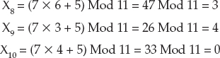
The RandomTrees program, shown in Figure 2-1, uses seed values to represent random trees. Enter a seed and click Go to generate a random tree. If two seed values differ by even 1, they produce very different results.
The RandomTrees program uses the seed value you enter to generate drawing parameters such as the number of branches the tree creates at each step, the angle at which the branches bend from their parent branch, and how much shorter each branch is than its parent. You can download the program from the book's website to see the details.
If you enter the same seed number twice, you produce the same tree both times.
Figure 2-1: Even slightly different seeds lead to very different random trees.
Cryptographically Secure PRNGs
Any linear congruential generator has a period over which it repeats, and that makes it unusable for cryptographic purposes.
For example, suppose you encrypt a message by using a PRNG to generate a value for each letter in the message and then adding that value to the letter. For example, the letter A plus 3 would be D, because D is three letters after A in the alphabet. If you get to Z, you wrap around to A. So, for example, Y + 3 = B.
This technique works quite well as long as the sequence of numbers is random, but a linear congruential generator has a limited number of seed values. All you need to do to crack the code is to try decrypting the message with every possible seed value. For each possible decryption, the program can look at the distribution of letters to see if the result looks like real text. If you picked the wrong seed, every letter should appear with roughly equal frequency. If you guessed the right seed, some letters, such as E and T, will appear much more often than other letters, such as J and X. If the letters are very unevenly distributed, you have probably guessed the seed.
This may seem like a lot of work, but on a modern computer it's not very hard. If the seed value is a 32-bit integer, only about 4 billion seed values are possible. A modern computer can check every possible seed in just a few seconds or, at most, minutes.
A cryptographically secure pseudorandom number generator (CSPRNG) uses more complicated algorithms to generate numbers that are harder to predict and to produce much longer sequences without entering a loop. They typically have much larger seed values. A simple PRNG might use a 32-bit seed. A CSPRNG might use keys that are 1,000 bits long to initialize its algorithm.
CSPRNGs are interesting and very “random,” but they have a couple of disadvantages. They are complicated, so they're slower than simpler algorithms. They also may not allow you to do all the initialization manually, so you may be unable to easily generate a repeatable sequence. If you want to use the same sequence more than once, you should use a simpler PRNG. Fortunately, most algorithms don't need a CSPRNG, so you can use a simpler algorithm.
Ensuring Fairness
Usually programs need to use a fair PRNG. A fair PRNG is one that produces all its possible outputs with the same probability. A PRNG that is unfair is called biased. For example, a coin that comes up heads two-thirds of the time is biased.
Many programming languages have methods that produce random numbers within any desired range. But if you need to write the code to transform the PRNG's values into a specific range, you need to be careful to do so in a fair way.
A linear congruential generator produces a number between 0 (inclusive) and M (exclusive), where M is the modulus used in the generator's equation:
![]()
Usually a program needs a random number within a range other than 0 to M. An obvious but bad way to map a number produced by the generator into a range Min to Max is to use the following equation:
![]()
For example, to get a value between 1 and 100, you would calculate the following:
![]()
The problem with this is that it may make some results more likely than others.
To see why, consider a small example where M = 3, Min = 0, and Max = 1. If the generator does a reasonable job, it produces the values 0, 1, and 2 with roughly equal probability. If you plug these three values into the preceding equation, you get the values shown in Table 2-1.
Table 2-1 PRNG Values and Results Mapped with a Modulus
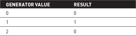
The result 0 occurs twice as often as the result 1 in Table 2-1, so the final result is biased.
In a real PRNG where the modulus M is very large, the problem is smaller, but it's still present.
A better approach is to convert the value produced by the PRNG into a fraction between 0 and 1 and then multiply that by the desired range, as in the following formula:
![]()
Another method of converting a pseudorandom value from one range to another is to simply ignore any results that fall outside the desired range. In the previous example, you would use the limited PRNG to generate a value between 0 and 2. If you get a 2, which is outside the desired range, you ignore it and get another number.
For a slightly more realistic example, suppose you want to give a cookie to one of four friends and you have a six-sided die. In that case you could simply roll the die repeatedly until you get a value between 1 and 4.
Getting Fairness from Biased Sources
Even if a PRNG is unfair, there may be a way to generate fair numbers. For example, suppose you think a coin is unfair. You don't know the probabilities of getting heads or tails, but you suspect the probabilities are not 0.5. In that case, the following algorithm produces a fair coin flip:
Flip the biased coin twice. If the result is {Heads, Tails}, return Heads. If the result is {Tails, Heads}, return Tails. If the result is something else, start over.
To see why this works, suppose the probability of the biased coin coming up heads is P, and the probability of its coming up tails is 1 − P. Then the probability of getting heads followed by tails is P × (1 − P). The probability of getting tails followed by heads is (1 − P) × P. The two probabilities are the same, so the probability of the algorithm returning heads or tails is the same, and the result is fair.
If the biased coin gives you heads followed by heads or tails followed by tails, you need to repeat the algorithm. If you are unlucky or the coin is very biased, you may need to repeat the algorithm many times before you get a fair result. For example, if P = 0.9, 81% of the time the coin will give you heads followed by heads, and 1% of the time it will give you tails followed by tails.
WARNING Using a biased coin to produce fair coin flips is unlikely to be useful in a real program. But it's a good use of probabilities and would make an interesting interview question, so it's worth understanding.
You can use a similar technique to expand the range of a PRNG. For example, suppose you want to give one of your five friends a cookie, and your only source of randomness is a fair coin. In that case, you can flip the coin three times and treat the results as a binary number with heads representing 1 and tails representing 0. For example, heads, tails, heads corresponds to the value 101 in binary, which is 5 in decimal. If you get a result that is outside the desired range (in this example, heads, heads, heads gives the result 111 binary or 8 decimal, which is greater than the number of friends present), you discard the result and try again.
In conclusion, the PRNG tools that come with your programming language are probably good enough for most programs. If you need better randomness, you may need to look at CSPRNGs. Using a fair coin to pick a random number between 1 and 100 or using a biased source of information to generate fair numbers are more useful under weird circumstances or as interview questions.
Randomizing Arrays
A fairly common task for programs is randomizing the items in an array. For example, suppose a scheduling program needs to assign employees to work shifts. If the program assigns the employees alphabetically, in the order in which they appear in the database, or in some other static order, the employee who always gets assigned to the late night shift will complain.
Some algorithms can also use randomness to prevent a worst-case situation. For example, the standard quicksort algorithm usually performs well but if the values it must sort are initially already sorted, the algorithm performs terribly. One way to avoid that situation would be to randomize the values before sorting them.
The following algorithm shows one way to randomize an array:
RandomizeArray(String: array[]) Integer: max_i = <Upper bound of array> For i = 0 To max_i - 1 // Pick the item for position i in the array. Integer: j = <pseudorandom number between i and max_i inclusive> <Swap the values of array[i] and array[j]> Next i End RandomizeArray
This algorithm visits every position in the array once, so it has a run time of O(N), which should be fast enough for most applications.
Note that repeating this algorithm does not make the array “more random.” When you shuffle a deck of cards, items that start near each other tend to remain near each other (although possibly less near each other), so you need to shuffle several times to get a reasonably random result. This algorithm completely randomizes the array in a single pass, so running it again just wastes time.
One other important consideration of this algorithm is whether it produces a fair arrangement. In other words, is the probability that an item ends up in any given position the same for all positions? For example, it would be bad if the item that started in the first position finished in the first position half of the time.
I said in the Introduction that this book doesn't include long mathematical proofs. So if you want, you can skip the following discussion and take my word for it that the randomness algorithm is fair. If you know some probability, however, you may find the discussion kind of interesting.
For a particular item in the array, consider the probability of its being placed in position k. To be placed in position k, it must not have been placed in positions 1, 2, 3,..., k − 1 and then placed in position k.
Define P−i to be the probability of the item's not being placed in position i given that it was not previously placed in positions 1, 2,..., i − 1. Also define Pk to be the probability of the item's being placed in position k given that it was not placed in positions 1, 2,..., k − 1. Then the total probability that the item is placed in position k is P−1 × P−2 × P−3 × ... × P−(k−1) × Pk.
P1 is 1 / N, so P−1 is 1 − P1 = 1 − 1 / N = (N − 1) / N.
After the first item is assigned, N − 1 items could be assigned to position 2, so P2 is 1 / (N − 1), and P−2 is 1 − P2 = 1 − 1 / (N − 1) = (N − 2) / (N −1).
More generally, Pi = 1 / (N − (i − 1)) and P−i = 1 − Pi = 1 − 1 / (N − (i − 1)) = (N − (i − 1) − 1) / (N − (i − 1)) = (N − i) / (N − i + 1).
If you multiply the probabilities together, P−1 × P−2 × P−3 × ... × P−(k−1) × Pk gives the following equation:
![]()
If you look at the equation, you'll see that the numerator of each term cancels out with the denominator of the following term. When you make all the cancelations, the equation simplifies to 1/N.
This means that the probability of the item's being placed in position k is 1/N no matter what k is, so the arrangement is fair.
A task very similar to randomizing an array is picking a certain number of random items from an array without duplication.
For example, suppose you're holding a drawing to give away five copies of your book (something I do occasionally), and you get 100 entries. One way to pick five names is to put the 100 names in an array, randomize it, and then give the books to the first five names in the randomized list. The probability that any particular name is in any of the five winning positions is the same, so the drawing is fair.
Generating Nonuniform Distributions
Some programs need to generate pseudorandom numbers that are not uniformly distributed. Often these programs simulate some other form of random-number generation. For example, a program might want to generate numbers between 2 and 12 to simulate the roll of two six-sided dice.
You can't simply pick pseudorandom numbers between 2 and 12, because you won't have the same probability of getting each number that you would get by rolling two dice.
The solution is to actually simulate the dice rolls by generating two numbers between 1 and 6 and adding them together.
Finding Greatest Common Divisors
The greatest common divisor (GCD) of two integers is the largest integer that evenly divides both of the numbers. For example, GCD(60, 24) is 12 because 12 is the largest integer that evenly divides both 60 and 24. (The GCD may seem like an esoteric function but it is actually quite useful in cryptographic routines that are widely used in business to keep such things as financial communications secure.)
NOTE If GCD(A, B) = 1, A and B are said to be relatively prime or coprime.
One way to find the GCD is to factor the two numbers and see which factors they have in common. However, the Greek mathematician Euclid recorded a faster method in his treatise Elements circa 300 BC. The following pseudocode shows the modern version of the algorithm. Because it is based on Euclid's work, this algorithm is called the Euclidian algorithm or Euclid's algorithm:
Integer: GCD(Integer: A, Integer: B) While (B != 0) Integer: remainder = A Mod B // GCD(A, B) = GCD(B, remainder) A = B B = remainder End While Return A End GCD
For example, consider GCD(4851, 3003). Table 2-2 shows the values for A, B, and A Mod B at each step.
Table 2-2: Values Used to Calculate GCD(4851, 3003)
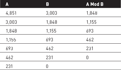
When B becomes 0, the variable A holds the GCD—in this example, 231. To verify the result, note that 4,851 = 231 × 21 and 1,848 = 231 × 8, so 231 divides both numbers. The values 21 and 8 have no common factors, so 231 is the largest integer that divides 4,851 and 1,848.
Great GCDs
This is another mathematical explanation that you can skip if you really want to.
The key to Euclid's algorithm is the fact that GCD(A, B) = GCD(B, A Mod B).
To understand why this is true, consider the definition of the modulus operator. If the remainder R = A Mod B, A = m × B + R for some integer m. If g is the GCD of A and B, g divides B evenly, so it must also divide m × B evenly. Because g divides A evenly and A = m × B + R, g must divide m × B + R evenly. Because g divides m × B evenly, it must also divide R evenly.
This proves that g divides B and R. To say g = GCD(B, R) you still need to know that g is the largest integer that divides B and R evenly.
Suppose G is an integer larger than g, and G divides B and R. Then G also divides m × B + R. But A = m × B + R, so G divides A as well. This means that g is not GCD(A, B). This contradicts the assumption that g = GCD(A, B). Because the assumption that G > g leads to a contradiction, there must be no such G, and g is GCD(A, B).
This algorithm is quite fast because the value B decreases by at least a factor of 1/2 for every two trips through the While loop. Because the size of B decreases by a factor of at least 1/2 for every two iterations, the algorithm runs in time at most O(log B).
The value B in Euclid's algorithm decreases by at least a factor of 1/2 for every two trips through the While loop. To see why, let Ak, Bk, and Rk be the A, B, and R values for the kth iteration, and consider A1 = m1 × B1 + R1 for some integer m1. In the second iteration, A2 = B1 and B2 = R1.
If R1 ≤ B1 / 2, B2 ≤ B1 / 2 as desired.
Suppose R1 > B1 / 2. In the third iteration, A3 = B2 = R1 and B3 = R2. By definition, R2 = A2 Mod B2, which is the same as B1 Mod R1. We're assuming that R1 > B1 / 2, so R1 divides into B1 exactly once with a remainder of B1 − R1. Because we're assuming that R1 > B1 / 2, we know that B1 − R1 ≤ B1 / 2. Working back through the equations:
B1 − R1 = B1 Mod R1 = A2 Mod B2 = R2 = B3
Therefore, B3 ≤ B1 / 2 as desired.
Performing Exponentiation
Sometimes a program needs to calculate a number raised to an integer power. That's not hard if the power is small. For example, 73is easy to evaluate by multiplying 7 × 7 × 7 = 343.
For larger powers such as 7102,187,291, however, this would be fairly slow.
NOTE Calculating large powers such as 7102,187,291 might be slow, but people probably wouldn't care very much if it weren't for the fact that this kind of large exponentiation is used in some important kinds of cryptography.
Fortunately, there's a faster way to perform this kind of operation. This method is based on two key facts about exponentiation:
- A2 × M = (AM)2
- AM+N = AM × AN
The first fact lets you quickly create powers of A where the power itself is a power of 2.
The second fact lets you combine those powers of A to build the result you want.
The following pseudocode shows the algorithm at a high level:
// Calculate A to the power P. Float: RaiseToPower(Float: A, Integer: P) <Use the first fact to quickly calculate A, A2, A4, A8, and so on until you get to a value AN where N + 1 > P> <Use those powers of A and the second fact to calculate AP> Return AP End RaiseToPower
For example, suppose you want to calculate 76. First the algorithm calculates 71, 72, and 74. It stops there because the next power, 8, is greater than the desired power, 6:
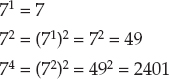
Next the algorithm uses the second fact to build 6 from the powers of 2 that are already created. If you think of 6 as being a sum of powers of 2, 6 = 2 + 4. Using the second fact, you know that 76 = 72 × 74 = 49 × 2,401 = 117,649.
Performing this calculation took two multiplications to calculate 72and 74 plus one more multiplication to find the final result, for a total of three multiplications. That's fewer multiplications than simply multiplying 7 × 7 × 7 × 7 × 7 × 7, but it's a small difference in this example.
More generally, for the exponent P, the algorithm calculates log(P) powers of A. It then examines the binary digits of A to see which of those powers it must multiply together to get the final result. (If a binary digit of P is 1, then the final result should include the corresponding power of 2. For the previous example, the binary representation of 6 is 110 so the second and third powers of 2 are included: 22 and 24.)
In binary, the value P has log2 (P) digits, so the total run time is O(log P) + O(log P) = O(log P). Even if P is 1 million, log(P) is about 20, so this algorithm uses about 20 steps (up to 40 multiplications), which is a lot fewer than 1 million.
One limitation of this algorithm is that values raised to large powers grow extremely large. Even a “small” value such as 7300 has 254 decimal digits. This means that multiplying the huge numbers needed to calculate large powers is slow and takes up quite a bit of space.
Fortunately, the most common applications for these kinds of huge powers are cryptographic algorithms that perform all their operations in a modulus. The modulus is large, but it still limits the numbers' size. For example, if the modulus has 100 digits, the product of two 100-digit numbers can have no more than 200 digits. You then reduce the result with the modulus to again get a number with no more than 100 digits. Reducing each number with the modulus makes each step slightly slower, but it means you can calculate values of practically unlimited size.
Working with Prime Numbers
As you probably know, a prime number is a counting number (an integer greater than 0) greater than 1 whose only factors are 1 and itself. A composite number is a counting number greater than 1 that is not prime.
Prime numbers play important roles in some applications where their special properties make certain operations easier or more difficult. For example, some kinds of cryptography use the product of two large primes to provide security. The fact that it is hard to factor a number that is the product of two large primes is what makes the algorithm secure.
The following sections discuss common algorithms that deal with prime numbers.
Finding Prime Factors
The most obvious way to find a number's prime factors is to try dividing the number by all the numbers between 2 and 1 less than the number. When a possible factor divides the number evenly, save the factor, divide the number by it, and continue trying more possible factors. Note that you need to try the same factor again before moving on in case the number contains more than one copy of the factor.
For example, to find the prime factors of 127, you would try to divide 127 by 2, 3, 4, 5, and so on until you reach 126.
The following pseudocode shows this algorithm:
List Of Integer: FindFactors(Integer: number) List Of Integer: factors Integer: i = 2 While (i < number) // Pull out factors of i. While (number Mod i == 0) // i is a factor. Add it to the list. factors.Add(i) // Divide the number by i. number = number / i End While // Check the next possible factor. i = i + 1 End While // If there's anything left of the number, it is a factor, too. If (number > 1) Then factors.Add(number) Return factors End FindFactors
If the number is N, this algorithm has run time O(N).
You can improve this method considerably with three key observations:
- You don't need to test whether the number is divisible by any even number other than 2 because, if it is divisible by any even number, it is divisible by 2. This means that you only need to check divisibility by 2 and then by odd numbers instead of by all possible factors. Doing so cuts the run time in half.
- You only need to check for factors up to the square root of the number. If n = p × q, either p or q must be less than or equal to sqrt(n). (If both are greater than sqrt(n), their product is greater than n.) If you check possible factors up to sqrt(n), you will find the smaller factor, and when you divide n by that factor, you will find the other one. This reduces the run time to O(sqrt(n)).
- Every time you divide the number by a factor, you can update the upper bound on the possible factors that you need to check.
These observations lead to the following improved algorithm:
List Of Integer: FindFactors(Integer: number) List Of Integer: factors // Pull out factors of 2. While (number Mod 2 == 0) factors.Add(2) number = number / 2 End While // Look for odd factors. Integer: i = 3 Integer: max_factor = Sqrt(number) While (i <= max_factor) // Pull out factors of i. While (number Mod i == 0) // i is a factor. Add it to the list. factors.Add(i) // Divide the number by i. number = number / i // Set a new upper bound. max_factor = Sqrt(number) End While // Check the next possible odd factor. i = i + 2 End While // If there's anything left of the number, it is a factor, too. If (number > 1) Then factors.Add(number) Return factors End FindFactors
NOTE This prime factoring algorithm has run time O(sqrt(N)), where N is the number it is factoring, so it is reasonably fast for relatively small numbers. If N gets really large, even O(sqrt(N)) isn't fast enough. For example, if N is 100 digits long, sqrt(N) has 50 digits. If N happens to be prime, even a fast computer won't be able to try all the possible factors in a reasonable amount of time. This is what makes some cryptographic algorithms secure.
Finding Primes
Suppose your program needs to pick a large prime number. (Yet another task required by some cryptographic algorithms.) One way to find prime numbers is to use the algorithm described in the preceding section to test a bunch of numbers to see if they are prime. For reasonably small numbers, that works, but for very large numbers, it can be prohibitively slow.
The sieve of Eratosthenes is a simple method of finding all the primes up to a given limit. This method works well for reasonably small numbers, but it requires a table with entries for every number that is considered. Therefore, it uses an unreasonable amount of memory if the numbers are too large.
The basic idea is to make a table with one entry for each of the numbers between 2 and the upper limit. Cross out all the multiples of 2 (not counting 2 itself). Then, starting at 2, look through the table to find the next number that is not crossed out (3 in this case). Cross out all multiples of that value (not counting the value itself). Note that some of the values may already be crossed out because they were also a multiple of 2. Repeat this step, finding the next value that is not crossed out, and cross out its multiples until you reach the square root of the upper limit. At that point, any numbers that are not crossed out are prime.
The following pseudocode shows the basic algorithm:
// Find the primes between 2 and max_number (inclusive). List Of Integer: FindPrimes(long max_number) // Allocate an array for the numbers. Boolean: is_composite = new bool[max_number + 1] // "Cross out" multiples of 2. For i = 4 to max_number Step 2 is_composite[i] = true Next i // "Cross out" multiples of primes found so far. Integer: next_prime = 3 Integer: stop_at = Sqrt(max_number) While (next_prime < stop_at) // "Cross out" multiples of this prime. For i = next_prime * 2 To max_number Step next_prime Then is_composite[i] = true Next i // Move to the next prime, skipping the even numbers. next_prime = next_prime + 2 While (next_prime <= max_number) And (is_composite[next_prime]) next_prime = next_prime + 2 End While End While // Copy the primes into a list. List Of Integer: primes For i = 2 to max_number If (Not is_composite[i]) Then primes.Add(i) Next i // Return the primes. Return primes End FindPrimes
It can be shown that this algorithm has run time O(N × log(log N)), but that is beyond the scope of this book.
Testing for Primality
The algorithm described in the earlier section “Finding Prime Factors” factors numbers. One way to determine whether a number is prime is to use that algorithm to try to factor it. If the algorithm doesn't find any factors, the number is prime.
As that section mentioned, that algorithm works well for relatively small numbers. But if the number has 100 digits, the number of steps the program must execute is a 50-digit number. Not even the fastest computers can perform that many operations in a reasonable amount of time. (A computer executing 1 trillion steps per second would need more than 3 × 1030years.)
Some cryptographic algorithms need to use large prime numbers, so this method of testing whether a number is prime won't work. Fortunately, there are other methods. The Fermat primality test is one of the simpler.
Fermat's “little theorem” states that if p is prime and 1 ≤ n ≤ p, np−1 Mod p = 1. In other words, if you raise n to the p−1 power and then take the result modulo p, the result is 1.
For example, suppose p = 11 and n = 2. Then np−1 Mod p = 210 Mod 11 = 1,024 Mod 11. The value 1,024 = 11 × 93 + 1, so 1,024 Mod 11 = 1 as desired.
Note that it is possible for np−1 Mod p = 1 even if p is not prime. In that case the value n is called a Fermat liar because it incorrectly implies that p is prime.
If np−1 Mod p ≠ 1, n is called a Fermat witness because it proves that p is not prime.
It can be shown that, for a natural number p, at least half of the numbers n between 1 and p are Fermat witnesses. In other words, if p is not prime and you pick a random number n between 1 and p, there is a 0.5 probability that n is a Fermat witness, so np−1 Mod p ≠ 1.
Of course, there is also a chance you'll get unlucky and randomly pick a Fermat liar for n. If you repeat the test many times, you can increase the chances that you'll pick a witness if one exists.
It can be shown that at each test there is a 50 percent chance that you'll pick a Fermat witness. So if p passes k tests, there is a 1/2k chance that you got unlucky and picked Fermat liars every time. In other words, there is a 1/2k chance that p is actually a composite number pretending to be prime.
For example, if p passes the test 10 times, there is a 1/210 ≈ 0.00098 probability that p is not prime. If you want to be even more certain, repeat the test 100 times. If p passes all 100 tests, there is only a 1/2100 ≈7.8 × 10⁻³¹ probability that p is not prime.
The following pseudocode shows an algorithm that uses this method to decide whether a number is probably prime:
// Return true if the number p is (probably) prime. Boolean: IsPrime(Integer: p, Integer: max_tests) // Perform the test up to max_tests times. For test = 1 To max_tests <Pick a pseudorandom number n between 1 and p (exclusive)> If (np-1 Mod p != 1) Then Return false Next test // The number is probably prime. // (There is a 1/2max_tests chance that it is not prime.) Return true End IsPrime
NOTE This is an example of a probabilistic algorithm—one that produces a correct result with a certain probability. There's still a slim chance that the algorithm is wrong, but you can repeat the tests until you reach whatever level of certainty you want.
If the number p is very large—which is the only time when this whole issue is interesting—calculating np−1 by using multiplication could take quite a while. Fortunately, you know how to do this quickly by using the fast exponentiation algorithm described in the earlier section “Performing Exponentiation.”
Once you know how to determine whether a number is (probably) prime, you can write an algorithm to pick prime numbers:
// Return a (probable) prime with max_digits digits. Integer: FindPrime(Integer: num_digits, Integer: max_tests) Repeat <Pick a pseudorandom number p with num_digits digits> If (IsPrime(p, max_tests)) Then Return p End FindPrime
Performing Numerical Integration
Numerical integration, which is also sometimes called quadrature or numeric quadrature, is the process of using numerical techniques to approximate the area under a curve defined by a function. Often the function is a function of one variable y = F(x) so the result is a two-dimensional area, but some applications might need to calculate the three-dimensional area under a surface defined by a function z = F(x, y). You could even calculate areas defined by higher-dimensional functions.
If the function is easy to understand, you may be able to use calculus to find the exact area. But perhaps you cannot find the function's antiderivative. For example, maybe the function's equation is complex, or you have data generated by some physical process, so you don't know the function's equation. In that case, you can't use calculus, but you can use numerical integration.
There are several ways to perform numerical integration. The most straightforward uses Newton-Cotes formulas, which use a series of polynomials to approximate the function. The two most basic kinds of Newton-Cotes formulas are the rectangle rule and the trapezoid rule.
The Rectangle Rule
The rectangle rule uses a series of rectangles of uniform width to approximate the area under a curve. Figure 2-2 shows the RectangleRule sample program (which is available for download on the book's website) using the rectangle rule. The program also uses calculus to calculate the exact area under the curve so that you can see how far the rectangle rule is from the correct result.
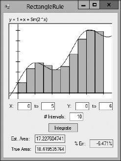
Figure 2-2: The RectangleRule sample program uses the rectangle rule to approximate the area under the curve y = 1 + x + Sin(2 × x).
The following pseudocode shows an algorithm for applying the rectangle rule:
Float: UseRectangleRule(Float: function(), Float: xmin, Float: xmax, Integer: num_intervals) // Calculate the width of a rectangle. Float: dx = (xmax - xmin) / num_intervals // Add up the rectangles' areas. Float: total_area = 0 Float: x = xmin For i = 1 To num_intervals total_area = total_area + dx * function(x) x = x + dx Next i Return total_area End UseRectangleRule
The algorithm simply divides the area into rectangles of constant width and with height equal to the value of the function at the rectangle's left edge. It then loops over the rectangles, adding their areas.
The Trapezoid Rule
Figure 2-2 shows where the rectangles don't fit the curve exactly, producing an error in the total calculated area. You can reduce the error by using more, skinnier rectangles. In this example, increasing the number of rectangles from 10 to 20 reduces the error from roughly −6.5% to −3.1%.
An alternative strategy is to use trapezoids to approximate the curve instead of using rectangles. Figure 2-3 shows the TrapezoidRule sample program (which is available for download on the book's website) using the trapezoid rule.
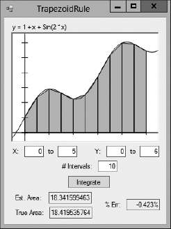
Figure 2-3: The TrapezoidRule sample program uses the trapezoid rule to make a better approximation than the RectangleRule program does.
The following pseudocode shows an algorithm for applying the trapezoid rule:
Float: UseTrapezoidRule(Float: function(), Float: xmin, Float: xmax, Integer: num_intervals) // Calculate the width of a trapezoid. Float: dx = (xmax - xmin) / num_intervals // Add up the trapezoids' areas. Float: total_area = 0 Float: x = xmin For i = 1 To num_intervals total_area = total_area + dx * (function(x) + function(x + dx)) / 2 x = x + dx Next i Return total_area End UseTrapezoidRule
The only difference between this algorithm and the rectangle rule algorithm is in the statement that adds the area of each slice. This algorithm uses the formula for the area of a trapezoid: area = width × average of the lengths of the parallel sides.
You can think of the rectangle rule as approximating the curve with a step function that jumps from one value to another at each rectangle's edge. The trapezoid rule approximates the curve with line segments.
Another example of a Newton-Cotes formula is Simpson's rule, which uses polynomials of degree 2 to approximate the curve. Other methods use polynomials of even higher degree to make better approximations of the curve.
Adaptive Quadrature
A variation on the numerical integration methods described so far is adaptive quadrature, in which the program detects areas where its approximation method may produce large errors and refines its method in those areas.
For example, look again at Figure 2-3. In areas where the curve is close to straight, the trapezoids approximate the curve very closely. In areas where the curve is bending sharply, the trapezoids don't fit as well.
A program using adaptive quadrature looks for areas where the trapezoids don't fit the curve well and uses more trapezoids in those areas.
The AdaptiveMidpointIntegration sample program, shown in Figure 2-4, uses the trapezoid rule with adaptive quadrature. When calculating the area of a slice, this program first uses a single trapezoid to approximate its area. It then breaks the slice into two pieces and uses two smaller trapezoids to calculate their areas. If the difference between the larger trapezoid's area and the sum of the areas of the smaller trapezoids is more than a certain percentage, the program divides the slice into two pieces and calculates the areas of the pieces in the same way.
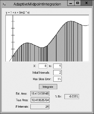
Figure 2-4: The AdaptiveMidpointIntegration program uses an adaptive trapezoid rule to make a better approximation than the TrapezoidRule program.
The following pseudocode shows this algorithm:
// Integrate by using an adaptive midpoint trapezoid rule. Float: IntegrateAdaptiveMidpoint(Float: function(), Float: xmin, Float: xmax, Integer: num_intervals, Float: max_slice_error) // Calculate the width of the initial trapezoids. Float: dx = (xmax - xmin) / num_intervals double total = 0 // Add up the trapezoids' areas. Float: total_area = 0 Float: x = xmin For i = 1 To num_intervals // Add this slice's area. total_area = total_area + SliceArea(function, x, x + dx, max_slice_error) x = x + dx Next i Return total_area End IntegrateAdaptiveMidpoint // Return the area for this slice. Float: SliceArea(Float: function(),Float: x1, Float: x2, Float: max_slice_error) // Calculate the function at the endpoints and the midpoint. Float: y1 = function(x1) Float: y2 = function(x2) Float: xm = (x1 + x2) / 2 Float: ym = function(xm) // Calculate the area for the large slice and two subslices. Float: area12 = (x2 - x1) * (y1 + y2) / 2.0 Float: area1m = (xm - x1) * (y1 + ym) / 2.0 Float: aream2 = (x2 - xm) * (ym + y2) / 2.0 Float: area1m2 = area1m + aream2 // See how close we are. Float: error = (area1m2 - area12) / area12 // See if this is small enough. If (Abs(error) < max_slice_error) Then Return area1m2 // The error is too big. Divide the slice and try again. Return SliceArea(function, x1, xm, max_slice_error) + SliceArea(function, xm, x2, max_slice_error) End SliceArea
If you run the AdaptiveMidpointIntegration program and start with only two initial slices, the program divides them into the 24 slices shown in Figure 2-4 and estimates the area under the curve with −0.035% error. If you use the TrapezoidRule program with 24 slices of uniform width, the program has an error of −0.072%, roughly twice as much as that produced by the adaptive program. The two programs use the same number of slices, but the adaptive program positions them more effectively.
The AdaptiveTrapezoidIntegration sample program uses a different method to decide when to break a slice into subslices. It calculates the second derivative of the function at the slice's starting x value and divides the interval into one slice plus 1 per second derivative value. For example, if the second derivative is 2, the program divides the slice into three pieces. (The formula for the number of slices was chosen somewhat arbitrarily. You might get better results with a different formula.)
NOTE In case your calculus is a bit rusty, a function's derivative tells you its slope at any given point. Its second derivative tells you the slope's rate of change, or how fast the curve is bending. A higher second derivative means that the curve is bending relatively tightly, so the AdaptiveTrapezoidIntegration program uses more slices.
Of course, this technique won't work if you can't calculate the curve's second derivative. The technique used by the AdaptiveMidpointIntegration program seems to work fairly well in any case, so you can fall back on that technique.
Adaptive techniques are useful in many algorithms because they can produce better results without wasting effort in areas where it isn't needed. The AdaptiveGridIntegration program shown in Figure 2-5 uses adaptive techniques to estimate the area in the shaded region. This region includes the union of vertical and horizontal ellipses, minus the areas covered by the three circles inside the ellipses.
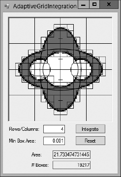
Figure 2-5: The AdaptiveGridIntegration program uses adaptive integration to estimate the area in the shaded region.
This program divides the whole image into a single box and defines a grid of points inside the box. In Figure 2-5 the program uses a grid with four rows and columns of points. For each point in the grid, the program determines whether the point lies inside or outside the shaded region.
If none of the points in the box lies within the shaded region, the program assumes the box is not inside the region and ignores it.
If every point in the box lies inside the shaded region, the program considers the box to lie completely within the region and adds the box's area to the region's estimated area.
If some of the points in the box lie inside the shaded region and some lie outside the region, the program subdivides the box into smaller boxes and uses the same technique to calculate the smaller boxes' areas.
In Figure 2-5, the AdaptiveGridIntegration program has drawn the boxes it considered so that you can see them. You can see that the program considered many more boxes near the edges of the shaded region than far inside or outside the region. In total, this example considered 19,217 boxes, mostly focused on the edges of the area it was integrating.
Monte Carlo Integration
Monte Carlo integration is form of numeric integration in which the program generates a series of pseudorandom points uniformly within an area and determines whether each point lies within the target region. When it has finished, the program uses the percentage of the points that were inside the region to estimate the region's total area.
For example, suppose the area within which the points are generated is a 20 × 20 square, so it has an area of 400 square units, and 37% of the pseudorandom points are within the region. The region has an area of roughly 0.37 × 400 = 148 square units.
The MonteCarloIntegration sample program shown in Figure 2-6 uses this technique to estimate the area of the same shape used by the AdaptiveGridIntegration program.
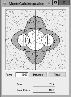
Figure 2-6: Points inside the shaded region are black, and points outside the region are gray.
Monte Carlo integration generally is more prone to error than more methodical approaches such as trapezoid integration and adaptive integration. But sometimes it is easier because it doesn't require you to know much about the nature of the shape you're measuring. You simply throw points at the shape and see how many hit it.
NOTE This chapter describes using pseudorandom values to calculate areas, but more generally you can use similar techniques to solve many problems. In a Monte Carlo simulation, you pick pseudorandom values and see what percentage satisfies some criterion to estimate the total number of values that satisfy the criterion.
Finding Zeros
Sometimes a program needs to figure out where an equation crosses the x-axis. In other words, given an equation y = f(x), you may want to find x where f(x) = 0. Values such as this are called the equation's roots.
Newton's method, which is sometimes called the Newton-Raphson method, is a way to successively approximate an equation's roots.
The method starts with an initial guess X0for the root. If f(X0) is not close enough to 0, the algorithm follows a line that is tangent to the function at the point X0 until the line hits the x-axis. It uses the x-coordinate at the intersection as a new guess X1 for the root.
The algorithm then repeats the process starting from the new guess X1. The algorithm continues the process of following tangents to the function to find new guesses until it finds a value Xk where f(Xk) is sufficiently close to 0.
The only tricky part is figuring out how to follow tangent lines. If you use a little calculus to find the derivative of the function f'(x), which is also written dfdx(x), the following equation shows how the algorithm can update its guess by following a tangent line:
![]()
NOTE Unfortunately, explaining how to find a function's derivative is outside the scope of this book. For more information, search online or consult a calculus book.
Figure 2-7 shows the process graphically. The point corresponding to the initial guess is labeled 1. That point's y value is far from 0, so the algorithm follows the tangent line until it hits the x-axis. It then calculates the function at the new guess to get the point labeled 2 in Figure 2-7. This point's y-coordinate is also far from 0, so the algorithm repeats the process to find the next guess, labeled 3. The algorithm repeats the process one more time to find the point labeled 4. Point 4's y-coordinate is close enough to 0, so the algorithm stops.
The following pseudocode shows the algorithm:
// Use Newton's method to find a root of the function f(x). Float: FindZero(Float: f(), Float: dfdx(), Float: initial_guess, Float: maxError) float x = initial_guess For i = 1 To 100 // Stop at 100 in case something goes wrong. // Calculate this point. float y = f(x) // If we have a small enough error, stop. if (Math.Abs(y) < maxError) break // Update x. x = x - y / dfdx(x) Next i Return x End NewtonsMethod
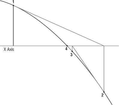
Figure 2-7: Newton's method follows a function's tangent lines to zero in on the function's roots.
The algorithm takes as parameters a function y = F(x), the function's derivative dfdx, an initial guess for the root's value, and a maximum acceptable error.
The code sets the variable x equal to the initial guess and then enters a For loop that repeats, at most, 100 times. Normally the algorithm quickly finds a solution. But sometimes, if the function has the right curvature, the algorithm can diverge and not zero in on a solution. Or it can get stuck jumping back and forth between two different guesses. The maximum of 100 iterations means the program cannot get stuck forever.
Within the For loop, the algorithm calculates F(x). If the result isn't close enough to 0, the algorithm updates x and tries again.
Note that some functions have more than one root. In that case, you need to use the FindZero algorithm repeatedly with different initial guesses to find each root.
Figure 2-8 shows the NewtonsMethod sample program, which is available for download on this book's website. This program uses Newton's method three times to find the three roots of the function y = x3 / 5 − x2 + x. Circles show the program's guesses as it searches for each root.
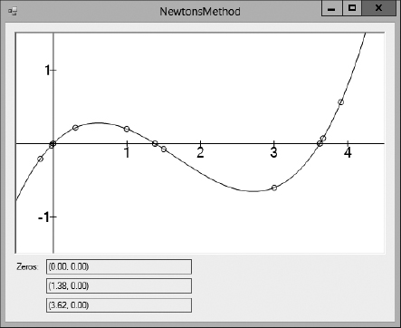
Figure 2-8: The NewtonsMethod sample program demonstrates Newton's method to find the three roots of the function y = x 3 / 5 − x2 + x.
Summary
Some numerical algorithms, such as randomization, are useful in a wide variety of applications. Other algorithms, such as prime factoring and finding the greatest common divisor, have more limited use. If your program doesn't need to find greatest common divisors, the GCD algorithm won't be much help.
However, the techniques and concepts demonstrated by these algorithms can be useful in many other situations. For example, the idea that an algorithm can be probabilistic is very important in many applications. That idea can help you devise other algorithms that don't work with perfect certainty (and that could easily be the subject of an interview question).
This chapter explained the ideas of fairness and bias, two very important concepts for any sort of randomized algorithm, such as the Monte Carlo integration algorithm, which also was described in this chapter.
This chapter also explained adaptive quadrature, a technique that lets a program focus most of its work on areas that are the most relevant and pay less attention to areas that are easy to manage. This idea of making a program adapt to spend the most time on the most important parts of the problem is applicable to many algorithms.
Many numerical algorithms, such as GCD, Fermat's primality test, the rectangle and trapezoid rules, and Monte Carlo integration, don't need complex data structures. In contrast, most of the other algorithms described in this book do require specialized data structures to produce their results. The next chapter explains one kind of data structure: linked lists. These are not the most complicated data structures you'll find in this book, but they are useful for many other algorithms. Also, the concept of linking data is useful in other data structures, such as trees and networks.
Exercises
Asterisks indicate particularly difficult problems.
- Write an algorithm to use a fair six-sided die to generate coin flips.
- The section “Getting Fairness from Biased Sources” explains how you can use a biased coin to get fair coin flips by flipping the coin twice. But sometimes doing two flips produces no result, so you need to repeat the process. Suppose the coin produces heads three-fourths of the time and tails one-fourth of the time. In that case, what is the probability that you'll get no result after two flips and have to try again?
- Again consider the coin described in Exercise 2. This time, suppose you were wrong, and the coin is actually fair but you're still using the algorithm to get fair flips from a biased coin. In that case, what is the probability that you'll get no result after two flips and have to try again?
- Write an algorithm to use a biased six-sided die to generate fair values between 1 and 6. How efficient is this algorithm?
- Write an algorithm to pick M random values from an array containing N items (where M ≤ N). What is its run time? How does this apply to the example described in the text where you want to give books to five people selected from 100 entries? What if you got 10,000 entries?
- Write an algorithm to deal five cards to players for a poker program. Does it matter whether you deal one card to each player in turn until every player has five cards, or whether you deal five cards all at once to each player in turn?
- Write a program that simulates rolling two six-sided dice and draws a bar chart or graph showing the number of times each roll occurs. Compare the number of times each value occurs with the number you would expect for two fair dice in that many trials. How many trials do you need to perform before the results fit the expected distribution well?
- What happens to Euclid's algorithm if A < B initially?
- The least common multiple (LCM) of integers A and B is the smallest integer that A and B both divide into evenly. How can you use the GCD to calculate the LCM?
- The fast exponentiation algorithm described in this chapter is at a very high level. Write a low-level algorithm that you could actually implement.
- How would you change the algorithm you wrote for Exercise 10 to implement modular fast exponentiation?
- *Write a program that calculates the GCD for a series of pairs of pseudorandom numbers and graphs the number of steps required by the GCD algorithm versus the average of the two numbers. Does the result look logarithmic?
- The following pseudocode shows how the sieve of Eratosthenes crosses out multiples of the prime next_prime:
// "Cross out" multiples of this prime. For i = next_prime * 2 To max_number Step next_prime Then is_composite[i] = true Next i
The first value crossed out is next_prime * 2. But you know that this value was already crossed out because it is a multiple of 2; the first thing the algorithm did was cross out multiples of 2. How can you modify this loop to avoid revisiting that value and many others that you have already crossed out?
- *In an infinite set of composite numbers called Carmichael numbers, every relatively prime smaller number is a Fermat liar. In other words, p is a Carmichael number if every n where 1 ≤ n ≤ p and GCD(p, n) = 1 is a Fermat liar. Write an algorithm to list the Carmichael numbers between 1 and 10,000 and their prime factors.
- When you use the rectangle rule, parts of some rectangles fall above the curve, increasing the estimated area, and other parts of some rectangles fall below the curve, reducing the estimated area. What do you think would happen if you used the function's value at the midpoint of the rectangle for the rectangle's height instead of the function's value at the rectangle's left edge? Write a program to check your hypothesis.
- Could you make a program that uses adaptive Monte Carlo integration? Would it be effective?
- Write a high-level algorithm for performing Monte Carlo integration to find the volume of a three-dimensional shape.
- How could you use Newton's method to find the points where two functions intersect?