CHAPTER 6

Sorting

There are several reasons why sorting algorithms are usually covered in great detail in algorithms books. First, they are interesting and demonstrate several useful techniques, such as recursion, problem subdivision, heaps, and trees.

Second, sorting algorithms are well studied and are some of the few algorithms for which exact run times are known. It can be shown that the fastest possible algorithm that uses comparisons to sort N items must use O(N log N) time. Several sorting algorithms actually achieve that performance, so in some sense they are optimal.

Finally, sorting algorithms are useful. Almost any data is more useful when it is sorted in various ways, so sorting algorithms play an important role in many applications.

This chapter describes several different sorting algorithms. Some, such as insertionsort, selectionsort, and bubblesort, are relatively simple but slow. Others, such as heapsort, quicksort, and mergesort, are more complicated but much faster. Still others, such as countingsort, don't use comparisons to sort items, so they can break the O(N log N) restriction and perform amazingly fast under the right circumstances.

The following sections categorize the algorithms by their run time performance.

O(N²) Algorithms

O(N²) algorithms are relatively slow but fairly simple. In fact, their simplicity sometimes lets them outperform faster but more complicated algorithms for very small arrays.

Insertionsort in Arrays

Chapter 3 describes an insertionsort algorithm that sorts items in linked lists, and Chapter 4 describes insertionsort algorithms that use stacks and queues. The basic idea is to take an item from the input list and insert it into the proper position in a sorted output list (which initially starts empty).

Chapter 3 explains how to do this in linked lists, but you can use the same steps to sort an array. The following pseudocode shows the algorithm for use with arrays:

As the code loops through the items in the array, the index i separates the items that have been sorted from those that have not. The items with an index less than i have already been sorted, and those with an index greater than or equal to i have not yet been sorted.

As i goes from 0 to the last index in the array, the code moves the item at index i into the proper position in the sorted part of the array.

To find the item's position, the code looks through the already sorted items and finds the first item that is greater than values[i]

The code then moves values[i] into its new position. This can be a time-consuming step. Suppose the item's new index should be j. In that case, the code must move the items between indices j and i one position to the right to make room for the item at position j.

Figure 6-1 shows the algorithm's key steps. The image at the top shows the original unsorted array. In the middle image, the first four items (outlined in bold) have been sorted, and the algorithm is preparing to insert the next item (which has value 3) into the sorted part of the array. The algorithm searches through the sorted items until it determines that the value 3 should be inserted before the value 5. At the bottom of the figure, the algorithm has moved the values 5, 6, and 7 to the right to make room for value 3. The algorithm inserts value 3 and continues the For loop to insert the next item (which has value 2) into its correct position.

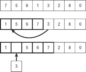
Figure 6-1: Insertionsort inserts items into the sorted part of the array.

This algorithm sorts the items in the original array, so it doesn't need any additional storage (aside from a few variables to control loops and move items).

If the array contains N items, the algorithm considers each of the N positions in the array. For each position i, it must search the previously sorted items in the array to find the ith item's new position. It must then move the items between that location and index i one position to the right. If the item i should be moved to position j, it takes j steps to find the new location j and then i – j more steps to move items over, resulting in a total of i steps. That means in total it takes i steps to move item i into its new position.

Adding up all the steps required to position all the items, the total run time is

This means the algorithm has run time O(N²). This isn't a very fast run time, but it's fast enough for reasonably small arrays (fewer than 10,000 or so items). It's also a relatively simple algorithm, so it may sometimes be faster than more complicated algorithms for very small arrays. How small an array must be for this algorithm to outperform more complicated algorithms depends on your system. Typically this algorithm is only faster for arrays holding 5 or 10 items.

Selectionsort in Arrays

In addition to describing insertionsort for linked lists, Chapter 3 also describes selectionsort for linked lists. Similarly Chapter 4 described selectionsort algorithms that use stacks and queues.

The basic idea is to search the input list for the largest item it contains and then add it to the end of a growing sorted list. Alternatively, the algorithm can find the smallest item and move it to the beginning of the growing list.

The following pseudocode shows the algorithm for use with arrays:

The code loops through the array to find the smallest item that has not yet been added to the sorted part of the array. It then swaps that smallest item with the item in position i.

Figure 6-2 shows the algorithm's key steps. The image at the top shows the original unsorted array. In the middle image, the first three items (outlined in bold) have been sorted, and the algorithm is preparing to swap the next item into position. The algorithm searches the unsorted items to find the one with the smallest value (3 in this case). The algorithm then swaps the item that has the smallest value into the next unsorted position. The image at the bottom of the figure shows the array after the new item has been moved to the sorted part of the array. The algorithm now continues the For loop to add the next item (which has value 5) to the growing sorted portion of the array.

Like insertionsort, this algorithm sorts the items in the original array, so it doesn't need any additional storage (aside from a few variables to control loops and move items).

If the array contains N items, the algorithm considers each of the N positions in the array. For each position i, it must search the N – i items that have not yet been sorted to find the item that belongs in position i. It then swaps the item into its final position in a small constant number of steps. Adding up the steps to move all the items gives the following run time:

This means the algorithm has run time O(N²), the same run time as insertionsort.

Like insertionsort, selectionsort is fast enough for reasonably small arrays (fewer than 10,000 or so items). It's also a fairly simple algorithm, so it may sometimes be faster than more complicated algorithms for very small arrays (typically 5 to 10 items).

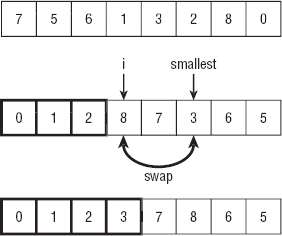
Figure 6-2: Selectionsort moves the smallest unsorted item to the end of the sorted part of the array.

Bubblesort

Bubblesort uses the fairly obvious fact that, if an array is not sorted, it must contain two adjacent elements that are out of order. The algorithm repeatedly passes through the array, swapping items that are out of order, until it can't find any more swaps.

The following pseudocode shows the bubblesort algorithm:

The code uses a boolean variable named not_sorted to keep track of whether it has found a swap in its most recent pass through the array. As long as not_sorted is true, the algorithm loops through the array, looking for adjacent pairs of items that are out of order, and swaps them.

Figure 6-3 shows an example. The array on the far left is mostly sorted. During the first pass through the array, the algorithm finds that the 6/3 pair is out of order (6 should come after 3), so it swaps 6 and 3 to get the second arrangement of values. During the second pass through the array, the algorithm finds that the 5/3 pair is out of order, so it swaps 5 and 3 to get the third arrangement of values. During the third pass through the array, the algorithm finds that the 4/3 pair is out of order, so it swaps 4 and 3, giving the arrangement on the far right in the figure. The algorithm performs one final pass, finds no pairs that are out of order, and ends.

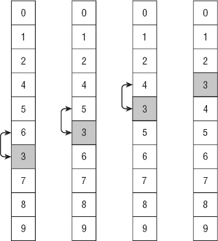
Figure 6-3: In bubblesort, items that are farther down than they should be slowly “bubble up” to their correct positions.

The fact that item 3 seems to slowly bubble up to its correct position gives the bubblesort algorithm its name.

During each pass through the array, at least one item reaches its final position. In Figure 6-3, item 6 reaches its final destination during the first pass, item 5 reaches its final destination during the second pass, and items 3 and 4 reach their final destinations during the third pass.

If the array holds N items and at least one item reaches its final position during each pass through the array, the algorithm can perform, at most, N passes. (If the array is initially sorted in reverse order, the algorithm needs all N passes.) Each pass takes N steps, so the total run time is O(N²).

Like insertionsort and selectionsort, bubblesort is fairly slow but may provide acceptable performance for small lists (fewer than 1,000 or so items). It is also sometimes faster than more complicated algorithms for very small lists (five or so items).

You can make several improvements to bubblesort. First, in Figure 6-3, the item with value 3 started out below its final correct position, but consider what happens if an item starts above its final position. In that case the algorithm finds that the item is out of position and swaps it with the following item. It then considers the next position in the array and finds the item again. If the item is still out of position, the algorithm swaps it again. The algorithm continues to swap that item down through the list until it reaches its final position in a single pass through the array. You can use this fact to speed up the algorithm by alternating downward and upward passes through the array. Downward passes quickly move items that are too high in the array, and upward passes quickly move items that are too low in the array.

To make a second improvement, notice that some items may move through several swaps at once. For example, during a downward pass, a large item (call it K) may be swapped several times before it reaches a larger item, and it stops for that pass. You can save a little time if you don't put item K back in the array for every swap. Instead, you can store K in a temporary variable and move other items up in the array until you find the spot where K stops. You then put K in that position and continue the pass through the array.

To make a final improvement, consider the largest item (call it L) that is not in its final position. During a downward pass, the algorithm reaches that item (possibly making other swaps beforehand) and swaps it down through the list until it reaches its final position. During the next pass through the array, no item can swap past L because L is in its final position. That means the algorithm can end its pass through the array when it reaches item L.

More generally, the algorithm can end its pass through the array when it reaches the position of the last swap it made during the previous pass. If you keep track of the last swaps made during downward and upward passes through the array, you can shorten each pass.

Figure 6-4 shows these three improvements. During the first pass down through the array, the algorithm swaps item 7 with items 4, 5, 6, and 3. It holds the value 7 in a temporary variable, so it doesn't need to save it back into the array until it reaches its final position.

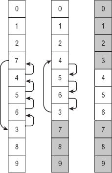
Figure 6-4: Improvements make bubblesort faster, but it still has O(N²) performance.

After placing 7 after 3, the algorithm continues moving through the array and doesn't find any other items to swap so it knows that item 7 and those that follow are in their final positions and don't need to be examined again. If some item nearer to the top of the array were larger than 7, the first pass would have swapped it down past 7. In the middle image shown in Figure 6-4, the final items are shaded to indicate that they don't need to be checked during later passes.

The algorithm knows item 7 and the items after it are in their final positions, so it starts its second pass, moving upward through the array at the first item before item 7, which is item 3. It swaps that item with items 6, 5, and 4, this time holding item 3 in a temporary variable until it reaches its final position.

Now item 3 and those that come before it in the array are in their final positions, so they are shaded in the last image in Figure 6-4.

The algorithm makes one final downward pass through the array, starting the pass at value 4 and ending at value 6. No swaps occur during this pass, so the algorithm ends.

These improvements make bubblesort faster in practice. (In one test sorting 10,000 items, bubblesort took 2.50 seconds without improvements and 0.69 seconds with improvements.) But it still has O(N²) performance, so there's a limit to the size of the list you can sort with bubblesort.

O(N log N) Algorithms

O(N log N) algorithms are much faster than O(N²) algorithms, at least for larger arrays. For example, if N is 1,000, N log N is less than 1×10⁴, but N² is roughly 100 times as big at 1×10⁶ . That difference in speed makes these algorithms more useful in everyday programming, at least for large arrays.

Heapsort

Heapsort uses a data structure called a heap and is a useful technique for storing a complete binary tree in an array.

Storing Complete Binary Trees in Arrays

A binary tree is a tree where every node is connected to, at most, two children. In a complete tree (binary or otherwise), all the tree's levels are completely filled, except possibly the last level, where all the nodes are pushed to the left.

Figure 6-5 shows a complete binary tree holding 12 nodes. The tree's first three levels are full. The fourth level contains five nodes pushed to the left side of the tree.

Figure 6-5: In a complete binary tree, every level is full, except possibly the last.

One useful feature of complete binary trees is that you can easily store them in an array using a simple formula. Start by placing the root node at index 0. Then, for any node with index i, place its children at indices 2 × i + 1 and 2 × i + 2.

If a node has index j, its parent has index (j − 1) / 2, where means to truncate the result to the next-smaller integer (round down). For example, 2.9 is 2, and 2 is also 2.

Figure 6-6 shows the tree shown in Figure 6-5 stored in an array, with the entry's indices shown on top.

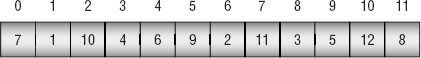
Figure 6-6: You can easily store a complete binary tree in an array.

For example, the value 6 is at index 4, so its children should be at indices 4 × 2 + 1 = 9 and 4 × 2 + 2 = 10. Those items have values 5 and 12. If you look at the tree shown in Figure 6-5, you'll see that those are the correct children.

If the index of either child is greater than the largest index in the array, the node doesn't have that child in the tree. For example, the value 9 has index 5. Its right child has index 2 × 5 + 2 = 12, which is beyond the end of the array. If you look at Figure 6-5, you'll see that the item with value 9 has no right child.

For an example of calculating a node's parent, consider the item with value 12 stored at index 10. The index of the parent is (10 − 1) / 2 = 4.5 = 4. The value at index 4 is 6. If you look at the tree shown in Figure 6-5, you'll see that the node with value 12 does have as its parent the node with value 6.

Defining Heaps

A heap, shown in Figure 6-7, is a complete binary tree where every node holds a value that is at least as large as the values in all its children. Figure 6-5 is not a heap because, for example, the root node has a value of 7, and its right child has a value of 10, which is greater.

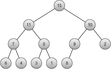
Figure 6-7: In a heap, the value of every node is at least as large as the values of its children.

You can build a heap one node at a time. Start with a tree consisting of a single node. Because it has no children, it satisfies the heap property.

Now suppose you have built a heap, and you want to add a new node to it. Add the new node at the end of the tree. There is only one place where you can add this node to keep the tree a complete binary tree—at the right end of the bottom level of the tree.

Now compare the new value to the value of its parent. If the new value is larger than the parent's, swap them. Because the tree was previously a heap, you know that the parent's value was already larger than its other child (if it has one). By swapping it with an even larger value, you know that the heap property is preserved at this point.

However, you have changed the value of the parent node, so that might break the heap property farther up in the tree. Move up the tree to the parent node, and compare its value to the value of its parent, swapping their values if necessary.

Continue up the tree, swapping values if necessary, until you reach the root node. At that point the tree is again a heap.

Figure 6-8 shows this process when you add the value 12 to the tree shown in Figure 6-7. Figure 6-9 shows the new heap.

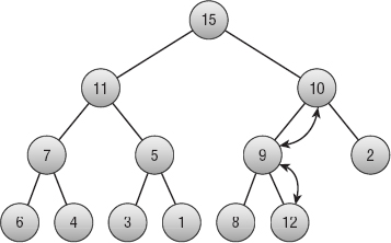
Figure 6-8: To add a new value to a heap, place the value at the end of the tree, and move it up as needed to restore the heap property.

Figure 6-9: When the value moves up to a node that already satisfies the heap property, the tree is once again a heap.

Storing the heap in an array makes this process particularly easy, because when you need to add a new item to the end of the tree, it's already in the proper position in the array.

The following pseudocode shows the algorithm to turn an array into a heap:

Heaps are useful for creating priority queues because the largest item in the tree is always at the root node. When you need to remove an item from the queue, you simply use the item at the root.

Unfortunately, that breaks the heap, so it is no longer a tree. Fortunately, there's an easy way to fix it: Move the last item in the tree to the root.

Doing so breaks the tree's heap property, but you can fix that using a method similar to the one you used to build the heap. If the new value is smaller than one of its child values, swap it with the larger child. That fixes the heap property at this node, but it may have broken it at the child's level, so move down to that node and repeat the process. Continue swapping the node down into the tree until you find a spot where the heap property is already satisfied or you reach the bottom of the tree.

The following pseudocode shows the algorithm to remove an item from the heap and restore the heap property:

This algorithm takes as a parameter the size of the tree, so it can find the location where the heap ends within the array.

The algorithm starts by saving the value at the root node so that it can return it later. It then moves the last item in the tree to the root node.

The algorithm sets the variable index to the index of the root node and then enters an infinite While loop.

Inside the loop, the algorithm calculates the indices of the children of the current node. If either of those indices is off the end of the tree, it is set to the current node's index. In that case, when the node's values are compared later, the current node's value is compared to itself. Because any value is greater than or equal to itself, that comparison satisfies the heap property, so the missing node does not make the algorithm swap values.

After the algorithm calculates the child indices, it checks whether the heap property is satisfied at this point. If it is, the algorithm breaks out of the While loop. (If both child nodes are missing, or if one is missing and the other satisfies the heap property, the While loop ends.)

If the heap property is not satisfied, the algorithm sets swap_child to the index of the child that holds the larger value and swaps the parent node's value with that child node's value. It then updates the index variable to move down to the swapped child node and continues down the tree.

Implementing Heapsort

Now that you know how to build and maintain a heap, implementing the heapsort algorithm is easy. The algorithm builds a heap. It then repeatedly swaps the first and last items in the heap, and rebuilds the heap excluding the last item. During each pass, one item is removed from the heap and added to the end of the array where the items are placed in sorted order.

The following pseudocode shows how the algorithm works:

This algorithm starts by turning the array of values into a heap. It then repeatedly removes the top item, which is the largest, and moves it to the end of the heap. It reduces the number of items in the heap and restores the heap property, leaving the newly positioned item at the end of the heap in its proper sorted order.

When it is finished, the algorithm has removed the items from the heap in largest-to-smallest order and placed them at the end of the ever-shrinking heap. The array is left holding the values in smallest-to-largest order.

The space required by heapsort is easy to calculate. The algorithm stores all the data inside the original array and uses only a fixed number of extra variables for counting and swapping values. If the array holds N values, the algorithm uses O(N) space.

The runtime required by the algorithm is slightly harder to calculate. To build the initial heap, the algorithm adds each item to a growing heap. Each time it adds an item, it places the item at the end of the tree and swaps the item upward until the tree is again a heap. Because the tree is a complete binary tree, it is O(log N) levels tall, so pushing the item up through the tree can take, at most, O(log N) steps. The algorithm performs this step of adding an item and restoring the heap property N times, so the total time to build the initial heap is O(N log N).

To finish sorting, the algorithm removes each item from the heap and then restores the heap property. It does that by swapping the last item in the heap and the root node, and then swapping the new root down through the tree until the heap property is restored. The tree is O(log N) levels tall, so this can take up to O(log N) time. The algorithm repeats this step N times, so the total number of steps required is O(N log N).

Adding the time needed to build the initial heap and the time to finish sorting gives a total time of O(N log N) + O(N log N) = O(N log N).

Heapsort is an elegant “sort-in-place” algorithm that takes no extra storage. It also demonstrates some useful techniques such as heaps and storing a complete binary tree in an array.

Even though heapsort's O(N log N) run time is asymptotically the fastest possible for an algorithm that sorts by using comparisons, the quicksort algorithm described in the next section usually runs slightly faster.

Quicksort

The quicksort algorithm works by subdividing an array into two pieces and then calling itself recursively to sort the pieces. The following pseudocode shows the algorithm at a high level:

For example, the top of Figure 6-10 shows an array of values to sort. In this case I picked the first value, 6, for divider.

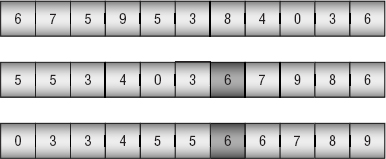
Figure 6-10: When the value moves up to a node that already satisfies the heap property, the tree is once again a heap.

In the middle image, values less than divider have been moved to the beginning of the array, and values greater than or equal to divider have been moved to the end of the array. The divider item is shaded at index 6. Notice that one other item has value 6, and it comes after the divider in the array.

The algorithm then calls itself recursively to sort the two pieces of the array before and after the divider item. The result is shown at the bottom of Figure 6-10.

Before moving into the implementation details, you should study the algorithm's run time behavior.

Analyzing Quicksort's Runtime

First, consider the special case in which the dividing item divides the part of the array that is of interest into two exactly equal halves at every step. Figure 6-11 shows the situation.

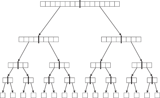
Figure 6-11: If the divider item divides the array into equal halves, the algorithm progresses quickly.

Each of the “nodes” in the tree shown in Figure 6-11 represents a call to the quicksort algorithm. The thick line in the middle of the node shows how the array was divided into two equal halves. The two arrows out of the node represent the quicksort algorithm calling itself twice to process the two halves.

The nodes at the bottom of the tree represent calls to sort a single item. Because a list holding a single item is already sorted, those calls simply return without doing anything.

After the calls work their way to the bottom of the tree, they begin returning to the methods that called them, so control moves back up the tree.

If the array originally holds N items and the items divide exactly evenly, as shown in Figure 6-11, the tree of quicksort calls is log N levels tall.

Each call to quicksort must examine all the items in the piece of the array it is sorting. For example, a call to quicksort represented by a group of four boxes in Figure 6-11 would need to examine those four boxes to further divide its values.

All the items in the original array are present at each level of the tree, so each level of the tree contains N items. If you add up the items that each call to quicksort must examine at any level of the tree, you get N items. That means the calls to quicksort on any level require N steps.

The tree is log N levels tall, and each level requires N steps, so the algorithm's total run time is O(N log N).

All this analysis assumes that the quicksort algorithm divides its part of the array into two equal-sized pieces at every step. In practice, that would be extremely unlikely.

Most of the time, however, the dividing item will belong somewhere more or less in the middle of the items it is dividing. It won't be in the exact middle, but it won't be near the edges either. For example, in Figure 6-10 the dividing item 6 ended up close to but not exactly in the middle in the second image. If the dividing item is usually somewhere near the middle of the values it is dividing, then in the expected case, the quicksort algorithm still has O(N log N) performance.

In the worst case, suppose the dividing item is less than any of the other items in the part of the array that it is dividing. (The worst case also occurs if all the items in the array have the same value.) In that case, none of the items goes into the left piece of the array, and all the other items (except the dividing item) go into the right piece of the array. The first recursive call returns immediately because it doesn't need to sort any items, but the second call must process almost all the items. If the first call to quicksort had to sort N items, this recursive call must sort N − 1 items.

If the dividing item is always less than the other items in the part of the array being sorted, the algorithm is called to sort N items, and then N − 1 items, and then N − 2 items, and so on. In that case the call tree shown in Figure 6-11 is extremely tall and thin, with a height of N.

The calls to quicksort at level i in the tree must examine N − i items. Adding up the items that all the calls must examine gives N + (N − 1) + (N − 2) + ... + 1 = N × (N + 1) / 2, which is O(N²), so the algorithm's worst-case behavior is O(N²).

In addition to examining the algorithm's run time performance, you should consider the space it needs. This depends partly on the method you use to divide parts of the array into halves, but it also depends on the algorithm's depth of recursion. If the sequence of recursive calls is too deep, the program will exhaust its stack space and crash.

For the tree shown in Figure 6-11, the quicksort algorithm calls itself recursively to a depth of log N calls. In the expected case, that means the program's call stack will be O(log N) levels deep. That shouldn't be a problem for most computers. Even if the array holds 1 billion items, log N is only about 30, and the call stack should be able to handle 30 recursive method calls.

For the tall thin tree created in the worst case, however, the depth of recursion is N. Few programs will be able to safely build a call stack with 1 billion recursive calls.

You can help avoid the worst-case scenario to make the algorithm run in a reasonable amount of time and with a reasonable depth of recursion by picking the dividing item carefully. The following section describes some strategies for doing so. The sections after that one describe two methods for dividing a section of an array into two halves. The final section discussing quicksort summarizes issues with using quicksort in practice.

Picking a Dividing Item

One method of picking the dividing item is to simply use the first item in the part of the array being sorted. This is quick, simple, and usually effective. Unfortunately if the array happens to be initially sorted or sorted in reverse, the result is the worst case. If the items are randomly arranged, this worst case behavior is extremely unlikely, but it seems reasonable that the array of items might be sorted or mostly sorted for some applications.

One solution is to randomize the array before calling quicksort. If the items are randomly arranged, it is extremely unlikely that this method will pick a bad dividing item every time and result in worst-case behavior. Chapter 2 explains how to randomize an array in O(N) time so that this won't add to quicksort's expected O(N log N) run time, at least in Big O notation. In practice it still could take a fair amount of time for a large array, however, so most programmers don't use this approach.

Another approach is to examine the first, last, and middle items in part of the array being sorted and use the value that is between the other two for the dividing item. This doesn't guarantee that the dividing item isn't close to the largest or smallest in this part of the array, but it does make it less likely.

A final approach is to pick a random index from the part of the array being sorted and then use the value at that index as the dividing item. It would be extremely unlikely that every such random selection would produce a bad dividing value and result in worst-case behavior.

Implementing Quicksort with Stacks

After you have picked a dividing item, you must divide the items into two sections to be placed at the front and back of the array. One easy way to do this is to move items into one of two stacks, depending on whether the item you are considering is greater than or less than the dividing item. The following pseudocode shows the algorithm for this step:

At this point, the algorithm is ready to recursively call itself to sort the two pieces of the array on either side of the dividing item.

Implementing Quicksort in Place

Using stacks to split the items in the array into two groups as described in the preceding section is easy, but it requires you to allocate extra space for the stacks. You can save some time if you allocate the stacks at the beginning of the algorithm and then let every call to the algorithm share the same stacks instead of creating their own, but this still requires the stacks to hold O(N) memory during their first use.

With a little more work, you can split the items into two groups without using any extra storage. The following high-level pseudocode shows the basic approach:

Continue looking backwards from the end of the array and forwards from the start of the array, moving items into the hole, until the two regions you are searching meet somewhere in the middle. Place the dividing item in the hole, which is now between the two pieces, and recursively call the algorithm to sort the two pieces.

This is a fairly confusing step, but the actual code isn't all that long. If you study it closely, you should be able to figure out how it works.

The following pseudocode shows the entire quicksort algorithm at a low level:

This algorithm starts by checking whether the section of the array contains one or fewer items. If it does, it is sorted, so the algorithm returns.

If the section of the array contains at least two items, the algorithm saves the first item as the dividing item. You can use some other dividing item selection method if you like. Just swap the dividing item you pick to the beginning of the section so that the algorithm can find it in the following steps.

Next the algorithm uses variables lo and hi to hold the highest index in the lower part of the array and the lowest index in the upper part of the array. It uses those variables to keep track of which items it has placed in the two halves. Those variables also alternately track where the hole is left after each step.

The algorithm then enters an infinite While loop that continues until the lower and upper pieces of the array grow to meet each other.

Inside the outer While loop, the algorithm starts at index hi and searches the array backward until it finds an item that should be in the lower piece of the array. It moves that item into the hole left behind by the dividing item.

Next the algorithm starts at index lo and searches the array forward until it finds an item that should be in the upper pieces of the array. It moves that item into the hole left behind by the previously moved item.

The algorithm continues searching backward and then forward through the array until the two pieces meet. At that point it puts the dividing item between the two pieces and recursively calls itself to sort the pieces.

Using Quicksort

If you divide the items in place instead of by using stacks, quicksort doesn't use any extra storage (beyond a few variables).

Like heapsort, quicksort has O(N log N) expected performance, although quicksort can have O(N²) performance in the worst case. Heapsort has O(N log N) performance in all cases, so it is in some sense safer and more elegant. But in practice quicksort is usually faster than heapsort, so it is the algorithm of choice for most programmers. It is also the algorithm that is used in most libraries. (The Java library uses mergesort, at least sometimes. The following section provides more information about mergesort, and the “Stable Sorting” sidebar in that section has information about why Java uses mergesort.)

In addition to greater speed, quicksort has another advantage over heapsort: it is parallelizable. Suppose a computer has more than one processor, which is increasingly the case these days. Each time the algorithm splits a section of the array into two pieces, it can make different processors sort the two pieces. Theoretically a highly parallel computer could use O(N) processors to sort the list in O(log N) time. In practice, most computers have a fairly limited number of processors (for example, two or four), so the run time would be divided by the number of processors, plus some additional overhead to manage the different threads of execution. That won't change the Big O run time, but it should improve performance in practice.

Because it has O(N²) performance in the worst case, the implementation of quicksort provided by a library may be cryptographically insecure. If the algorithm uses a simple dividing item selection strategy, such as picking the first item, an attacker might be able to create an array holding items in an order that gives worst-case performance. The attacker might be able to launch a denial-of-service (DOS) attack by passing your program that array and ruining your performance. Most programmers don't worry about this possibility, but if this is a concern, you can use a randomized dividing item selection strategy.

Mergesort

Like quicksort, mergesort uses a divide-and-conquer strategy. Instead of picking a dividing item and splitting the items into two groups holding items that are larger and smaller than the dividing item, mergesort splits the items into two halves of equal size. It then recursively calls itself to sort the two halves. When the recursive calls to mergesort return, the algorithm merges the two sorted halves into a combined sorted list.

The following pseudocode shows the algorithm:

In addition to the array to sort and the start and end indices to sort, the algorithm also takes as a parameter a scratch array that it uses to merge the sorted halves.

This algorithm starts by checking whether the section of the array contains one or fewer items. If it does, it is trivially sorted, so the algorithm returns.

If the section of the array contains at least two items, the algorithm calculates the index of the item in the middle of the section of the array and recursively calls itself to sort the two halves.

Next the algorithm merges the two sorted halves. It loops through the halves, copying the smaller item from whichever half holds it into the scratch array. When one half is empty, the algorithm copies the remaining items from the other half.

Finally, the algorithm copies the merged items from the scratch array back into the original values array.

The “call tree” shown in Figure 6-11 shows calls to quicksort when the values in the array are perfectly balanced, so the algorithm divides the items into equal halves at every step. The mergesort algorithm does divide the items into exactly equal halves at every step, so Figure 6-11 applies even more to the mergesort algorithm than it does to quicksort.

The same run time analysis shown earlier for quicksort also works for mergesort, so this algorithm also has O(N log N) run time. Like heapsort, mergesort's run time does not depend on the initial arrangement of the items, so it always has O(N log N) run time and doesn't have a disastrous worst case like quicksort does.

Like quicksort, mergesort is parallelizable. When a call to mergesort calls itself recursively, it can make one of those calls on another processor. This requires some coordination, however, because the original call must wait until both recursive calls finish before it can merge their results. In contrast, quicksort can simply tell its recursive calls to sort a particular part of the array, and it doesn't need to wait until those calls return.

Mergesort is particularly useful when all the data to be sorted won't fit in memory at once. For example, suppose a program needs to sort 1 million customer records, each of which occupies 1 MB. Loading all that data into memory at once would require 10¹⁸ bytes of memory, or 1,000 TB, which is much more than most computers have.

The mergesort algorithm, however, doesn't need to load that much memory all at once. The algorithm doesn't even need to look at any of the items in the array until after its recursive calls to itself have returned.

At that point, the algorithm walks through the two sorted halves in a linear fashion and merges them. Moving through the items linearly reduces the computer's need to page memory to and from disk. When quicksort moves items into the two halves of a section of an array, it jumps from one location in the array to another, increasing paging and greatly slowing down the algorithm.

Mergesort was even more useful in the days when large data sets were stored on tape drives, which work most efficiently if they keep moving forward with few rewinds. (Sorting data that cannot fit in memory is called external sorting.) Specialized versions of mergesort were even more efficient for tape drives. They're interesting but not commonly used anymore, so they aren't described here.

A more common approach to sorting enormous data sets is to sort only the items' keys. For example, a customer record might occupy 1 MB, but the customer's name might occupy only 100 bytes. A program can make a separate index that matches names to record numbers and then sort only the names. Then, even if you have 1 million customers, sorting their names requires only about 100 MB of memory, an amount that a computer could reasonably hold. (Chapter 11 describes B-trees and B+ trees, which are often used by database systems to store and sort record keys in this manner.)

Sub O(N log N) Algorithms

Earlier this chapter said that the fastest possible algorithm that uses comparisons to sort N items must use at least O(N log N) time. Heapsort and mergesort achieve that bound, and so does quicksort in the expected case, so you might think that's the end of the sorting story. The loophole is in the phrase “that uses comparisons.” If you use a method other than comparisons to sort, you can beat the O(N log N) bound.

The following sections describe two algorithms that sort in less than O(N log N) time.

Countingsort

Countingsort works if the values you are sorting are integers that lie in a relatively small range. For example, if you need to sort 1 million integers with values between 0 and 1,000, countingsort can provide amazingly fast performance.

The basic idea behind countingsort is to count the number of items in the array that have each value. Then it is relatively easy to copy each value, in order, the required number of times back into the array.

Then the following pseudocode shows the countingsort algorithm:

The max_value parameter gives the largest value in the array. (If you don't pass it in as a parameter, the algorithm can figure it out by looking through the array.)

Let M be the number of items in the counts array (so M = max_value + 1) and let N be the number of items in the values array, If your programming language doesn't automatically initialize the counts array so that it contains 0s, the algorithm spends M steps initializing the array. It then takes N steps to count the values in the array.

The algorithm finishes by copying the values back into the original array. Each value is copied once, so that part takes N steps. If any of the entries in the counts array is still 0, the program also spends some time skipping over that entry. In the worst case, if all the values are the same, so that the counts array contains mostly 0s, it takes M steps to skip over the 0 entries.

That makes the total run time O(2 × N + M) = O(N + M). If M is relatively small compared to N, this is much smaller than the O(N log N) performance given by heapsort and the other algorithms described previously.

In one test, quicksort took 4.29 seconds to sort 1 million items with values between 0 and 1,000, but it took countingsort only 0.03 seconds. Note that this is a bad case for quicksort, because the values include lots of duplicates. With 1 million values between 0 and 1,000, roughly 1,000 items have each value, and quicksort doesn't handle lots of duplication well.

With similar values, heapsort took roughly 1.02 seconds. This is a big improvement on quicksort but still is much slower than countingsort.

Bucketsort

The bucketsort algorithm (also called bin sort) works by dividing items into buckets. It sorts the buckets either by recursively calling bucketsort or by using some other algorithm and then concatenates the buckets' contents back into the original array. The following pseudocode shows the algorithm at a high level:

If the values in an array holding N items are reasonably uniformly distributed, if you use M buckets, and if the buckets divide the range of values evenly, you should expect roughly N / M items per bucket.

For example, consider the array shown at the top of Figure 6-12, which contains 10 items with values between 0 and 99. In the distribution step, the algorithm moves the items into the buckets. In this example, each bucket represents 20 values: 0 to 19, 20 to 39, and so on. In the sorting step, the algorithm sorts each bucket. The gathering step concatenates the values in the buckets to build the sorted result.

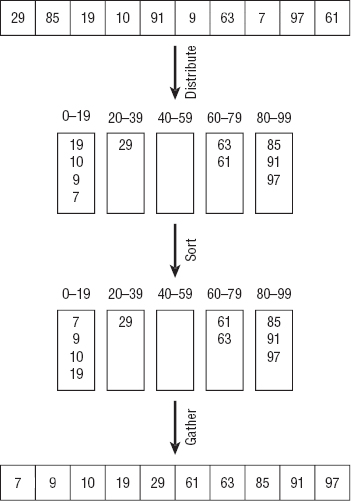
Figure 6-12: Bucketsort moves items into buckets, sorts the buckets, and then concatenates the buckets to get the sorted result.

The buckets can be stacks, linked lists, queues, arrays, or any other data structure that you find convenient.

If the array contains N fairly evenly distributed items, distributing them into the buckets requires N steps times whatever time it takes to place an item in a bucket. Normally this mapping can be done in constant time. For example, suppose the items are integers between 0 and 99, as in the example shown in Figure 6-12. You would place an item with value v in bucket number v / 20. You can calculate this number in constant time, so distributing the items takes O(N) steps.

If you use M buckets, sorting each bucket requires an expected F(N / M) steps, where F is the run time function of the sorting algorithm that you use to sort the buckets. Multiplying this by the number of buckets M, the total time to sort all the buckets is O(M × F(N / M)).

After you have sorted the buckets, gathering their values back into the array requires N steps to move all the values. It could require an additional O(M) steps to skip empty buckets if many of the buckets are empty, but if M < N, the whole operation requires O(N) steps.

Adding the times needed for the three stages gives a total run time of O(N) + O(M × F(N / M)) + O(N) = O(N + M × F(N / M)).

If M is a fixed fraction of N, N / M is a constant, so F(N / M) is also a constant, and this simplifies to O(N + M).

In practice, M must be a relatively large fraction of N for the algorithm to perform well. If you are sorting 10 million records and you use only 10 buckets, you need to sort buckets containing an average of 1 million items each.

Unlike countingsort, bucketsort's performance does not depend on the range of the values. Instead, it depends on the number of buckets you use.

Summary

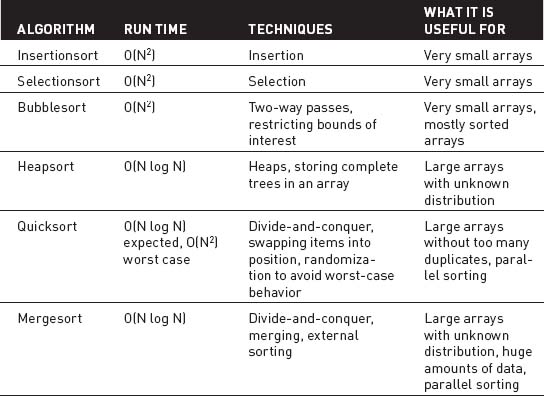
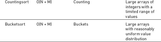
The sorting algorithms described in this chapter demonstrate different techniques and have different characteristics. Table 6-1 summarizes the algorithms.

Table 6-1: Algorithm Characteristics

These algorithms demonstrate an assortment of useful techniques and provide good performance for a wide variety of problems, but they're far from the end of the story. There are dozens of other sorting algorithms. Some are minor modifications of these algorithms, and others use radically different approaches. Chapter 10 discusses trees, which are also extremely useful for sorting data. Search the Internet for other algorithms.

This chapter explained several ways to sort data but didn't explain why you should want to do that. Simply having data sorted often makes it more useful to a user. Viewing customer accounts sorted by balance makes it much easier to determine which accounts need special attention.

Another good reason to sort data is so that you can later find specific items within it. For example, if you sort customers by their names, it's easier to locate a specific customer. The next chapter explains methods you can use to search a sorted set of data to find a specific value.

Exercises

1. Write a program that implements insertionsort.
2. The For i loop used by the insertionsort algorithm runs from 0 to the array's last index. What happens if it starts at 1 instead of 0? Does that change the algorithm's run time?
3. Write a program that implements selectionsort.
4. What change to selectionsort could you make that corresponds to the change described in Exercise 2? Would it change the algorithm's run time?
5. Write a program that implements bubblesort.
6. Add the first and third bubblesort improvements described in the section “Bubblesort” (downward and upward passes, and keeping track of the last swap) to the program you built for Exercise 5.
7. Write a program that uses an array-based heap to build a priority queue. So that you don't need to resize the array, allocate it at some fixed size, perhaps 100 items, and then keep track of the number of items that are used by the heap. (To make the queue useful, you can't just store priorities. Use two arrays—one to store string values, and another to store the corresponding priorities. Order the items by their priorities.)
8. What is the run time for adding items to and removing items from a heap-based priority queue?
9. Write a program that implements heapsort.
10. Can you generalize the technique used by heapsort for holding a complete binary tree so that you can store a complete tree of degree d? Given a node's index p, what are its children's indices? What is its parent's index?
11. Write a program that implements quicksort with stacks. (You can use the stacks provided by your programming environment or build your own.)
12. Write a program that implements quicksort with queues instead of stacks. (You can use the queues provided by your programming environment or build your own.) Is there any advantage or disadvantage to using queues instead of stacks?
13. Write a program that implements quicksort with in-place partitioning.
14. Quicksort can display worst-case behavior if the items are initially sorted, if the items are initially sorted in reverse order, or if the items contain many duplicates. You can avoid the first two problems if you choose random dividing items. How can you avoid the third problem?
15. Write a program that implements countingsort.
16. If an array's values range from 100,000 to 110,000, allocating a counts array with 110,001 entries would slow down countingsort considerably, particularly if the array holds a relatively small number of items. How could you modify countingsort to give good performance in this situation?
17. If an array holds N items that span the range 0 to M − 1, what happens to bucketsort if you use M buckets?
18. Write a program that implements bucketsort. Allow the user to specify the number of items, the maximum item value, and the number of buckets.
19. For the following data sets, which sorting algorithms would work well, and which would not?
    1. 10 floating-point values
    2. 1,000 integers
    3. 1,000 names
    4. 100,000 integers with values between 0 and 1,000
    5. 100,000 integers with values between 0 and 1 billion
    6. 100,000 names
    7. 1 million floating-point values
    8. 1 million names
    9. 1 million integers with uniform distribution
    10. 1 million integers with nonuniform distribution