
Chapter five
Polymer Flooding–Pilot Design

In this chapter, general guidelines for designing a polymer injection pilot will be provided. Best practices will also be discussed to make the most out of any injection trial.
5.1. Reservoir Screening – Reminder
Given the current recovery factors (averaging 35% oil originally in place (OOIP) after waterflood), there is a high potential for enhanced oil recovery (EOR) in brownfields, using existing infrastructure to facilitate the implementation. General guidelines were provided in Chapter 4 to assess the feasibility of polymer injection in a field. The two principal screening rules for polymer flooding are:
- Pointing out reservoirs that have poor sweep efficiency due to high oil viscosity and/or large‐scale heterogeneity.
- Determining whether the overall conditions are suitable (i.e. compatible brine, mobile oil saturation, retention) for polymer flooding implementation to fix the problem.
Polymer flooding has been applied in both sandstone and carbonate reservoirs. Because injection in carbonates requires a good reservoir understanding and thorough laboratory studies to find the most efficient chemistry, only sandstone reservoirs will be considered here; however, the main screening parameters apply to carbonates as well.
We can narrow the primary parameters needed to check whether polymer flooding is a viable option, by order of importance:
Table 0
| Parameter | Preferred condition |
| Lithology | Sandstones preferred |
| Wettability | Water‐wet |
| Current oil saturation | Above residual oil saturation |
| Porosity type (matrix/fractures) | Matrix preferred |
| Gas cap | See comments |
| Aquifer | Edge aquifer tolerated |
| Salinity/hardness | See comments |
| Dykstra‐Parsons and facies variations | 0.1 < DP < 0.8 |
| Clays | Low (see comments) |
| Water‐cut | See comments |
| Flooding pattern and spacing | Confined – small spacing |
The presence of clays can result in detrimental polymer loss within the reservoir, but solutions exist to minimize their impact on polymer efficiency. The potentially high salinity of the injection water is not a show‐stopper but will obviously impact the choice of chemistry and the dosage required to reach the target viscosity.
If screened reservoirs meet these criteria, there is a good chance that polymer flooding is technically viable. The next question is, is it economically viable? This aspect is very dependent on the particular field and should be discussed case by case.
5.2. Pilot Design
The first step to de‐risk the technology and evaluate the possible benefits is a pilot test. The primary goals of this approach are the following:
- Prove the technology/concept.
- Obtain valuable information about injection rates, pressure, optimum viscosity, etc.
- Check quality control procedures.
- Have operations personnel work directly with the technology and equipment to better understand the full‐scale requirements.
- Check the logistics, delivery, and supply chain.
- Use the information to update the reservoir model.
- Assess the economics of the project.
- Evaluate the produced water treatment technologies.
A pilot will not necessarily break even and should not be designed as such. Proving a concept sometimes requires an innovative approach to de‐risk as many parameters as possible and find the optimum injection strategy for full‐field deployment (Figure 5.1).
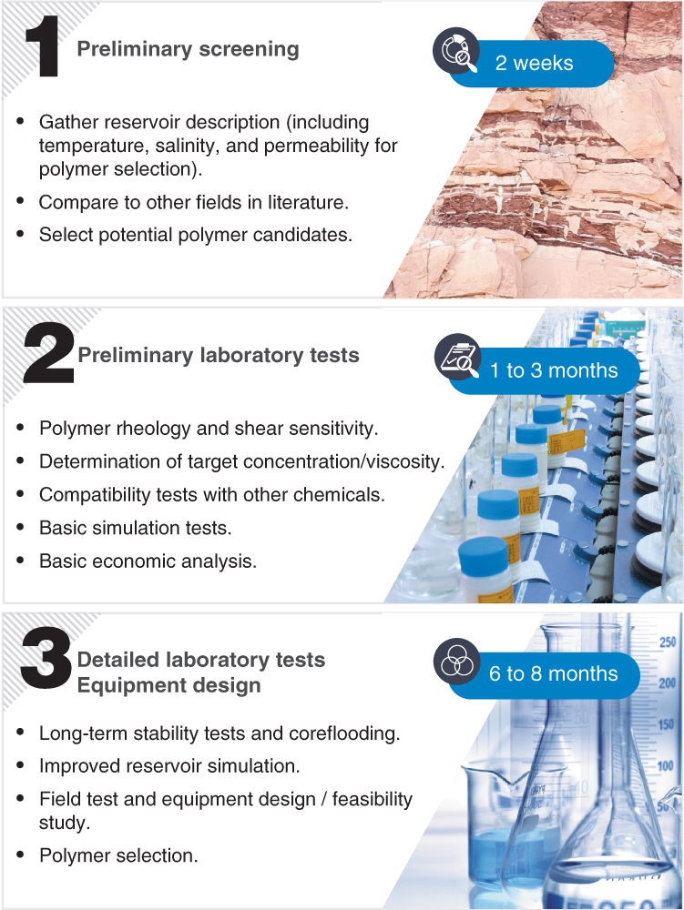

Figure 5.1 Polymer flooding: from design to implementation
5.2.1. Pattern Selection
Once a reservoir with acceptable characteristics has been chosen and polymer flooding is deemed applicable, the design can start. The first step consists of selecting the most appropriate zone for pilot injection. This decision is based on two main parameters:
- Finding a zone that is relatively representative of the entire reservoir.
- Minimizing the response time to obtain valuable information, in order to quickly decide on long‐lead items and begin the approval process for a full‐field expansion.
The response time varies based on many factors including spacing, reservoir thickness, injection rates, production history, etc. The general ideas are as follows:
- Select a confined pattern where the oil production from polymer injection can be isolated. For example: for vertical wells, five spots with a central producer; and for horizontal wells, two injection wells and one producer.
- Optimize the spacing to maximize efficiency. For verticals, a spacing between 100 and 150 m is preferred. For horizontals, a length of 1000 m maximum and a spacing of 100 m are suitable options. If the distance is less, early polymer breakthrough may impact efficiency.
- Check the connectivity between the wells (tracer tests, pressure tests, production history, and so on).
- If the reservoir is multilayered, if possible, isolate a zone for injection.
- Select a zone far from the water‐oil contact. If this is not possible, study the possibility of recompleting the well and isolating the zone.
- Check well completion and cleanliness. For cased vertical wells, a minimum of 12 perforations per foot is needed to minimize shear through the completion. Big bore (diameter and length) perforations can be used to further increase surface area for injection and reduce sandface shear. Acid jobs can be performed to clean the wells before the start of injection. For horizontals, perforated liners or wedge‐wrapped screens can be used with minimum degradation.
A detailed pattern analysis can be continued once the number of candidates has been narrowed using these criteria (Figure 5.2).

Figure 5.2 Five‐spot and inverted five‐spot patterns
5.2.2. How Much Polymer?
Defining a target viscosity (we should even say a resistance factor) is usually a prerequisite before starting any laboratory study or pilot design. If the reservoir is heterogeneous, with crossflow between layers, a calculation using Darcy's law shows that the ideal viscosity is equal to
The permeability contrast can be simply defined as the higher permeability divided by the lower permeability for adjacent layers with crossflow. In a case where no crossflow occurs, this term can be removed from the equation and only the mobility ratio considered. Seright [1] details the Daqing case where the end‐point mobility ratio is 10 and the permeability contrast is 4, yielding an optimum polymer viscosity of 40 cP. Obviously, in some heavy oil pools, this strategy is barely applicable, given the viscosity needed and the associated costs (not including injectivity aspects). But when possible, the mobility ratio value targeted should be less than 1, to take heterogeneities into account [2].
The volume of polymer injected is also very important. A rule of thumb is that at least 30% (or 50% in heavy oil pools) of the reservoir pore volume should be filled with polymer. However, from a reservoir engineering standpoint, and for good efficiency, the more the better. In Daqing, 60% of the reservoir has been filled with polymer; the volume is 80% in Mangala oil field (India), 50% in Shengli oil field (China), and 60% in Suffield (Canada) [1]. Stopping the injection depends largely on economics. When the cost of injecting polymer exceeds the benefits coming from the oil production, the process should cease [1], or a slug with a viscosity taper can be implemented to protect the back end of the entire polymer slug. A producer can be shut in when the water‐cut increases again to uneconomical values. If only 30% of pore volume has been injected, but oil is produced at economical rates, polymer injection should be continued. From a technical standpoint:
- A small polymer bank will not be efficient for recovering bypassed oil. When switching back to water, the water will not push the polymer slug homogeneously toward the producer but rather will finger through it in the high‐permeability zones, where the residual resistance factor is lowest. The consequences can even be worse if crossflow occurs.
- A large polymer bank can compensate for retention and maintain viscosity during the entire transit through the reservoir.
Additionally, in heterogeneous reservoirs, the size of the bank injected will have a huge impact on the following:
- The choice of the polymer. In theory, the polymer will be effective – and therefore should be stable – only over the portion of the reservoir injected. As stated earlier, when switching back to water, it will finger through the slug and dilute it. This should help determine the optimum chemistry from both a technical and an economic standpoint.
- The concentration of polymer that can be expected at the production side. If less than 1 pore volume is injected, the dilution effect caused by water injection and polymer retention in the virgin parts of the reservoir will reduce polymer concentration. Therefore, it is highly unlikely that the original polymer concentration will ever be seen in production wells. In cases where rapid tracer transit profiles exist, where fractures from injector and producer may be connected, or in close‐spacing horizontal injector/producer pairs with severe channeling, early polymer breakthroughs of high concentration can occur. The immediate result may be that the well
- must be shut in and that polymer injection can be continued only after a conformance treatment. If the produced polymer is being diluted by large produced brine volumes, it may not be an issue; however, the ability to produce to temporary tanks may minimize production facility upsets if they occur. This should be understood when designing the water treatment facilities and when health, safety, and environment (HSE) concerns are raised for offshore implementation.
Simulation studies and sensitivity analyses can be performed to optimize bank size, determine the impact of water chase on slug integrity, and evaluate the benefits of injecting a higher‐viscosity polymer plug.
Once the parameters have been set, it is possible to design the injection protocol and set a list of variables that should be monitored during the injection.
5.2.3. Injection Protocol
5.2.3.1. Start‐Up of Polymer Injection
Before the start of injection, the injection wells should be cleaned to allow good injectivity. When injecting in a mature reservoir, it is paramount to have a good water injection baseline, with stable injection rates and pressures to compare with polymer injection. There are different ways to start a polymer injection:
- Begin with the same injection rate as waterflood, and progressively increase the viscosity while monitoring reservoir response: for instance, one‐third of target viscosity, then two‐thirds, and finally target viscosity.
- Begin with a target viscosity of one‐third the target injection rate, then two‐thirds, and finally the full injection rate.
The first strategy helps obtain a good understanding of the flow regime, differentiating between linear and radial/matrix flow. In theory, if the flow is radial, an increase in viscosity from 1 to 2 cP at a given rate should lead to almost 50% injectivity loss (compared to water; see Section 5.3). If all injection guidelines to prevent polymer degradation have been respected, and if no significant injectivity loss is observed, then microfractures are likely present (see Section 5.3).
Hall plots can be used to monitor the reservoir response (see Section 5.4). If pressure does not stabilize and reservoir integrity is threatened, the best strategy is to decrease the injection rate without adjusting the viscosity.
Ending Polymer Injection
No clear rule defines how to stop polymer injection, but, generally speaking, two approaches are possible:
- Polymer injection is simply stopped, and water injection is resumed.
- Polymer viscosity is ramped down over a period of time to minimize mobility contrast between the polymer slug and chase water. In theory, this should help slightly delay water breaking through the slug and reaching the producers.
However, in both cases, once water injection is resumed, there is a high risk that the water‐cut will rise rapidly in the producers, along with small fractions of the injected polymer, which can occur over a very long period.
5.2.3.3. Voidage Replacement Ratio (VRR)
The voidage replacement ratio (VRR) is the ratio of reservoir barrels of injected fluid to reservoir barrels of produced fluid. Balancing injection and production is a common reservoir management practice for conventional oil‐bearing formations. Recent studies [3 4] and analyses have suggested, for heavy oils, that targeting a VRR below 1 could improve recovery by:
- Allowing compaction in compressible formations.
- Decreasing reservoir pressure and using a secondary gas‐cap drive.
Other authors have discussed this topic and shown that no clear correlations could be made with current field data, especially for Pelican Lake, where comprehensive information is available [5]. The compaction/dilation effect was also studied for a specific field in Suriname, showing that the injection strategy was indeed important, in addition to reservoir characteristics (heterogeneity), to explain the results observed in the field. The conclusions of the work were that there is an optimum rate, pressure, and viscosity to flood compressible formations. High injection rates could result in pressure and energy waste, dilating the formation and impairing oil displacement [6]. Other possible issues with VRR < 1 include the following:
- If more fluid is drawn, it will be difficult to pressurize the reservoir, leaving injection wells under vacuum in some cases. Pressure is therefore not a good indicator of the efficiency of polymer injection.
- Water fingers are likely to form when VRR < 1, bypassing large volumes of oil. When switching to polymer injection, given the pressure gradient, the slug might enter these zones preferentially, with deteriorated efficiency and, possibly, early polymer breakthrough.
In conclusion, the injection strategy depends on the reservoir and field constraints. A thorough reservoir analysis is required to understand all the parameters that influence oil recovery. For polymer injection, it is recommended, when possible, to balance injection and production; this will help with understanding the changes in fluid production and will enhance history matching.
A reservoir management strategy to maximize oil recovery may consist of purposefully building reservoir pressure at the start of polymer injection. For example, a strategy for a simple newly drilled pattern with two horizontal injectors and a central producer could be as follows:
- Shut in the producer.
- Inject a viscous polymer solution in both injection wells, quickly building pressure until the maximum allowable pressure is reached, indicating reservoir fill‐up. This pressure is usually mandated by the governments or determined from the reservoir fracture gradient and is monitored to not compromise reservoir and cap rock integrity.
- Open the producer.
- Decrease the injection rate slightly, keeping relatively low injection rates to minimize polymer breakthrough.
This strategy has the advantage of building a homogeneous polymer front in the injection well, maximizing the reservoir length contacted and minimizing the formation of water/polymer fingers. An obvious drawback is the absence of fluid production during pressure build‐up. This time can be shortened by optimizing the spacing and injection strategy.
5.3. Injectivity
Concerns about injectivity issues are often raised, since a viscous solution is injected instead of water [7]. Mathematically speaking, the injectivity index, II, is defined as:

where Q = injection rate (std bbl/d); P bhi = bottom‐hole pressure; P e = reservoir pressure (in psi); k w = permeability (mD); μ w = water viscosity (cp); B w = water formation volume factor (res vol/ST vol) r w and r e are the wellbore and drainage radii, respectively (ft); h i = injection height (ft); and S = total near‐wellbore skin.
Looking at this equation, there are two important parameters for polymer injection: bottom‐hole pressure and viscosity. It is very difficult to know these values precisely at any point in the injection facilities, especially in the well and the near‐wellbore area, for these reasons:
- Polymer solutions are non‐Newtonian fluids, so viscosity changes with the shear rate applied. In the well, where the shear is relatively high, viscosity will be low, which will also have an impact on the pressure drop during flow.
- Polymers act as friction reducers [8]. For the same injection rate, the pressure drop in the pipes when injecting polymer may be 70% less than with water. Therefore, predicting the pressure drop in the pipes and the pressure at the bottom‐hole will be difficult. Care should be taken when attempting to run a 3D model to predict injectivity (Figure 5.3).

Figure 5.3 Pressure drop average vs. Reynolds number in a 4″ pipe. Comparison between water and a polymer solution @10cP at 7,34 s−1
A clarification is required regarding the definition of an injectivity issue. Given the previous equation and polymer injection, an injectivity issue it translates into a decrease of the injected volume into a given reservoir, compared to waterflood. Let's consider three cases:
- Injectivity decreases dramatically right away upon commencement of polymer injection. There could be several reasons, including water quality, a damaged wellbore, or an abrupt change in fluid flow due to viscosity. In any case, the first response is to decrease the injection rate, keeping the same viscosity, to see if the pressure stabilizes. If the pressure does not stabilize, polymer injection should cease, the reasons should be investigated, and the well should be cleaned with
- Water only, at first. If the pressure doesn't decrease, then …
- Add an oxidizer or a chemical not compatible with the polymer, to break/degrade the molecule (sodium persulfate, bleach, or tetrakis hydroxymethyl phosphonium sulfate [THPS]). Conventional acid will not remove the polymer. If pressure still doesn't decrease (and the polymer is not at fault), then it is likely that solids, oil carry‐over, or a combination with the polymer is the cause of the observed injectivity decrease. At that stage, conventional acids can be considered.
- If the damage is too severe (fine migration, internal filter cake), fracturing may be required to restore injectivity.
- Injectivity decreases after a time. This should normally occur if the polymer slug mobilizes an oil bank: in that case, the pressure will slowly build up, possibly forcing a decrease in injection rate depending on reservoir and facility constraints. However, when the VRR is less than 1, pressure buildup in the reservoir may take a very long time and, in some cases, may not happen at all.
- Injectivity barely changes or increases. Several explanations are possible:
- Friction reduction effect, changing the pressure drop and mathematically affecting the injectivity index.
- Fracture extension and/or creation.
- Increase in the surface/area swept. If the flooding front enlarges, there is less pressure drop per linear meter.
- Viscosity loss due to degradation. Increasing the concentration temporarily will increase the viscosity, which can help detect changes. Also, variations in water‐cut or oil cuts can prove that viscosity remains in the reservoir, is sweeping more than before, and is mobilizing an oil bank.
- Injection out of zone (gas cap or water aquifer) and other issues related to reservoir management.
Looking at all existing and past projects, published or not, very few cases have been reported where an injectivity decrease was observed at the start of polymer injection. A probable reason is the presence of microfractures in the near‐wellbore area created during the well's drilling/completion or during water injection (or injection of cold water into a hot reservoir). Some existing flow paths are beneficial to polymer injection, in that microfractures can be extended slightly, decreasing the shear rate in the near‐wellbore area and therefore minimizing possible mechanical degradation [9, 10] . In some specific cases, it is also possible to pre‐shear the polymer solution to remove very‐high‐molecular‐weight molecules and enhance injectivity. However, some benefits may be lost, such as viscoelasticity. One last method to improve polymer injectivity is hot‐polymer injection, whereby the polymer is warmed prior to injection and viscosity in the near‐wellbore area is low; as the polymer flows further from the wellbore, it is cooled in the reservoir, gaining in situ viscosity.
5.3.1. Discussion on Injectivity
Understanding what happens in the near‐wellbore area is critical to the success of polymer injection. To build a business case, it is necessary to make predictions about the volumes injected and assume that the viscosity will remain intact during the project. In the near‐wellbore area, the main risk is mechanical degradation, either through perforations or at the sand face.
First, a differentiation should be made between vertical and horizontal injectors. Very often, the characteristics of horizontal wells make them good candidates for polymer injection: their length is important and the injection rate is not very high, especially onshore in shallow reservoirs. The area available for flow is therefore important, with low shear rates and little chance of mechanical degradation. Authors have also discussed the impact of completion [11], compaction/dilation, and fracture propagation in unconsolidated formations [12]. It is also possible to calculate the shear through orifices for completion with screens.
For verticals, completion is critical to ensure that little to no degradation occurs. The length and diameter of the perforation can be maximized to reduce shear; and the more perforations, the better (>12 shots per foot). But understanding the flow regime is also critical: the pressure drop and shear rate will not be the same if fractures exist.
Well tests and basic monitoring can help understand what happens in the well. First, it is necessary to obtain a steady water‐injection baseline and test reservoir pressure limits. Hall plots combined with pressure tests and other monitoring tools (step rate test) should be used to determine the parting pressure and set a maximum allowable pressure limit not to cross to minimize fracture propagation.
Another simple tool consists of analyzing injectivity through the value q/ΔP:


Where q = injection rate (barrels per day [BPD]), P = pressure drawdown (psi), k = permeability (md), h = formation height (ft), μ = fluid viscosity (cp), r e = external drainage radius (ft), and r w = wellbore radius (ft).
In order for this relationship to prove useful, very accurate measurements of the bottom‐hole injection and reservoir pressures should be known. In addition, flow capacity can be best represented if the injection well in question has been cored.
A careful review of existing field cases shows that most of the injections (water and polymer) were done under fracturing conditions [9, 10 13–15]. Several reasons can be given;
- Drilling a well changes the stresses around the bore, damaging the formation and weak zones.
- For cased, cemented, and perforated vertical wells, the perforation creates a fracture. The injected fluids will simply make the fracture propagate over time.
- In some cases, cold water injected into hot reservoirs can initiate thermal fractures.
Given these possibilities, there is little chance that polymer will encounter the rock matrix immediately after the perforations.
The best way to check injectivity is to run a trial with polymer: injecting a relatively low viscosity will give information about the flow regime. In theory, if the flow is radial, the following equation can be used to predict injectivity, relatively to water:

with I/I 0 = injectivity relative to water; r p = radius of polymer front (ft); r e = external drainage radius (ft); r w (wellbore radius); and F r = resistance factor.
In that case, given an external drainage radius of 1000 ft, a wellbore radius of 0.3 ft and a resistance factor for polymer of 2 (1 for water), we obtain the plot of I/I 0 versus radius of polymer front shown in Figure 5.4.
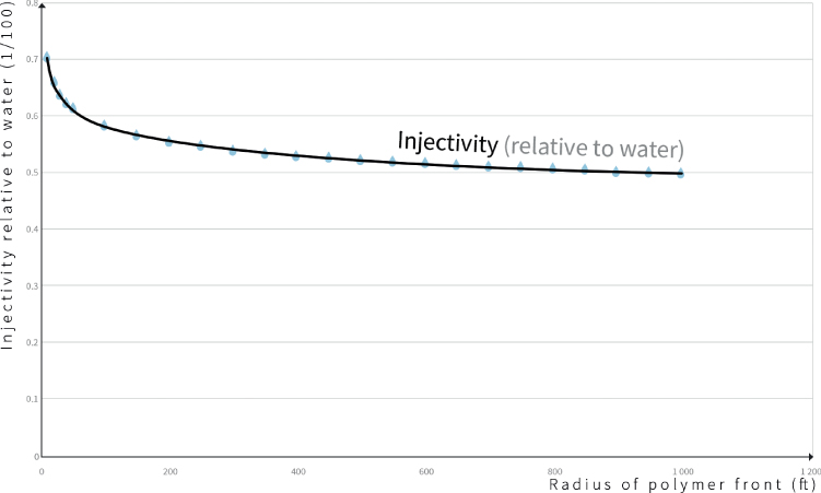
Figure 5.4 Injectivity relative to water, assuming no fractures (external drainage radius = 1000 ft, wellbore radius = 0.3 ft; resistance factor = 2)
Assuming no fractures, injectivity relative to water should decrease by 50% just by increasing the resistance factor from 1 to 2. First, this has never been observed in any field case documented. Second, if, during the trial, such a decrease is not observed, then it is likely the flow is not purely radial and microfractures exist. Such a test can be performed at a low injection rate to create favorable conditions for the polymer, to minimize potential mechanical degradation.
If fractures exist, there are important consequences:
- The pressure drop – and therefore shear – are dramatically decreased in linear flow, limiting polymer mechanical degradation [1].
- The shear‐thickening behavior disappears. Shear‐thickening is a phenomenon observed in the laboratory at very high flow rates in a core (matrix flow). When polymer molecules are forced through pores at high shear, the resistance factor greatly increases, to a point that mechanical degradation occurs. In the field, if fractures are present (no matrix flow), the surface opened to flow is much higher, and the polymer molecules encounter less resistance. Moreover, as shown in Figure 5.5, shear decreases very quickly once the fluid enters the reservoir, rapidly leaving the region where shear‐thickening could have occurred. Correlating fracture length with shear rate in the near‐wellbore area is therefore a good way to de‐risk mechanical degradation.

Figure 5.5 Shear vs. distance from the wellbore
Using microfractures or forcing their creation will help minimize mechanical degradation and maintain reasonable injection rates. Obviously, their extension should be controlled such that there is no direct connection between the injector and producer; the maximum distance should not be equal to more than one‐third the spacing. Fracture propagation can be followed with pressure and tracer tests, for instance. If rapid connection is observed, the injection rate should be decreased to allow partial closure of the fracture.
A thorough geomechanical analysis is also a good tool to understand fracture propagation and directions (vertical, horizontal, new versus reopened): geological properties of the reservoir, layering, facies, reservoir production history, reservoir depth, and injection rates will often limit fracture propagation (fluid leak‐off). Considerable information can be gathered from the hydraulic fracturing industry, where many efforts have been undertaken to understand fracture initiation and growth in tight formations. Below a certain depth, fractures grow vertically. Their growth will be limited by other geological formations or barriers, and there will be an increasing loss of fluid as it leaks into the most permeable zones [16]. In many formations, fracturing can be envisioned as similar to shattered glass, creating a complex fracture network that follows heterogeneities and whose extension is rapidly limited by fluid leak‐off (Figure 5.6).
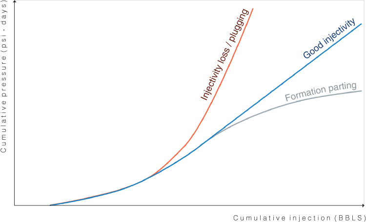
Figure 5.6 Hall plot – general description
Changes at the production side are another aspect that should be considered when discussing injectivity and injection rates. If the injection rate is decreased, but, at the production side, the oil‐cut and water‐cut percentages are switched in favor of oil production, then an economic balance can be reached. Here is a simple example: assume a void replacement ratio of 1 with 100 m3 d−1 water injected and 100 m3 d−1 of total fluid produced. If the water‐cut is 95% during the waterflood, then only 5 m3 d−1 of oil are produced. Now assume a decrease of 25% injectivity during polymer injection, and keep a void replacement ratio of 1; the total fluid injected and produced equal 75 m3 d−1. Assuming a decrease in water‐cut of 10% down to 85%, this translates to oil production of more than 11 m3 d−1, doubling the rate during waterflood. The fact that water‐cut decreases has a significant economic impact, since less water has to be treated and/or disposed of.
5.4. Monitoring
Before polymer injection, several tests can be performed to gain a better understanding of the reservoir and near‐wellbore area. These tests are also paramount for establishing a good baseline before switching to polymer injection. Typical tests include the following:
- Step rate tests (to determine parting pressure).
- Pressure fall‐off and pressure build‐up (injectivity/productivity, effective reservoir properties, and in situ polymer viscosity).
- Pulse tests (to check well connectivity).
- Production logging tool (PLT) (to identify the main reservoir units and reservoir conformance).
- Tracer tests (to check well connectivity and identify heterogeneities).
- Saturation logs (to ensure enough oil is left; also useful in surfactant‐polymer [SP] and alkali‐surfactant‐polymer [ASP] design).
Water quality can be monitored in conjunction with probes for oxygen and salinity (conductivity), and periodic sampling for iron content. The level of contaminants should be clearly determined to adapt the injection strategy, water treatment facilities, and choice of polymer and its protective package (if required).
During polymer injection, pressure and injection rates are usually continuously recorded at the injection side. The Hall plot, shown in Figure 5.6, can be used to track trends and detect either plugging or fracture formation. At the production side, parameters such as total fluid produced, water‐cut, and oil‐cut should be recorded. In the long term, for a brownfield, we should look at the following:
- Peak oil rate, breadth of peak, and response time to flood.
- Average oil rate and oil cut after peak response.
- Average sustained oil rate and oil cut to current date of flood.
- Average early injection rates.
- Sustained injection rates.
- Time before water breakthrough.
- Total oil recovered during the pilot.
In theory, the results of a pilot (total oil recovered) should be analyzed once the water‐cut again reaches the economic limit (98% or 99%).
5.5. Modeling
3D modeling is a useful tool that can help predict the efficiency of polymer flooding, assuming the user has a good understanding of polymer physics and flow properties. The most critical part is modeling the near‐wellbore area to duplicate the results observed in the field during pilot injection. Two runs should be made and their differences analyzed:
- Injection with a fixed bottom‐hole pressure. Usually, the injection rate will be limited quickly by the simulator because of increased viscosity, even though this is often not observed in the field.
- Injection with a fixed rate, close to the waterflood rate. This run will probably be closer to the actual field data, given the rheology of the solution and near‐wellbore features that usually are not accounted for (fractures, drag reduction, improved sweep efficiency, etc.).
Keywords related to shear‐thinning or shear‐thickening properties should be used carefully, with a good understanding of the wells' completion and the presence of damages or fractures. The most important parameters that can be obtained from laboratory experiments are resistance factors and retention. If no porous‐media experiment has been performed, it is possible to use the low‐shear viscosity obtained in conventional rheometers for simulation purposes, since, in the middle of the reservoir, the polymer solution will likely show Newtonian behavior given the low shear rates. Polymer degradation in the reservoir is usually limited, since the chemistry is always selected to remain stable during propagation throughout the reservoir. Input can be gathered from long‐term stability tests. A conservative approach should be taken for the residual resistance factor, using a value of 1. Sensitivity analyses should be made of slug size and viscosity, based on the water chase and a low Rk value, as mentioned earlier.
The model should be updated during the pilot injection and the results used to build the true business case.
5.6. Quality Control
The most important parameter in polymer flooding remains viscosity. Not everything can be controlled or anticipated, but many precautions can be taken to minimize the risk of degradation. If all engineering guidelines (for both surface facilities and well completions) are respected, along with close monitoring of water quality, then chances are that the viscosity will remain intact when entering the reservoir. There are currently two ways to control viscosity at the wellhead:
- Manual sampling
- Inline viscosity monitoring
If not carried out properly, manual sampling can lead to polymer degradation due to the following:
- Oxygen ingress during sampling and/or viscosity measure‐ment.
- Mechanical degradation resulting from the way the sample is taken or the sampling device itself, i.e. excess pressure drop across a valve or orifice.
Specific sampling methods and devices have been developed to avoid degradation during sampling and the measurement itself. The main drawback of manual sampling is manpower. To solve this problem, inline viscometers have been developed that display the viscosity value in real time [17]. Discrepancies from expected viscosity values can be observed quickly and actions taken to remedy the problem.
Product quality can be controlled with standard tests such as yield‐viscosity determination and filter ratio. All indications are provided in the certificate of analysis along with procedures to verify that the product falls within the specifications.
5.7. Specific Considerations for Offshore Implementation
The design of polymer injection offshore is complex for several reasons. The first is footprint. When infrastructure is already in place, space and weight limitations often make the installation of new equipment complicated. This aspect, together with local constraints (weather and marine conditions), will dictate the choice of product form (powder or emulsion). The second aspect is related to the presence of devices such as chokes, which are difficult to replace or change and can dramatically degrade the polymer solution. Solutions exist that can still make the process viable:
- Chemical solutions. Adapt the polymer chemistry and molecular weight, or develop delayed‐action polymers that will uncoil once in the reservoir.
- Mechanical solutions. Non‐shearing chokes can replace the existing ones or be part of greenfield development.
A third aspect that impacts polymer injection is well spacing. Offshore, the residence time in the reservoir is quite long, and the response time is a matter of years. Without a decrease in spacing to get faster results, little can be done to accelerate the process:
- EOR should be started on day 1 to minimize fingering and unwanted water production.
- Viscosity can be increased to play on the conformance effect and also limit retention and degradation and improve sweep while delaying polymer breakthrough.
- A large enough pore volume should be injected to offset retention and delay water breakthrough during the final water chase.
The fact that distances are very significant drives people to choose very robust chemistries, always assuming that the polymer will be efficient all the way from the injection well to the producer. With current developments and new chemistries, polymers have robust designs that provide good stability. What might not be stable is the displacement of the polymer slug by the water chase, which will render the process inefficient and the use of expensive chemistries not completely justified. A compromise should be found to minimize expenses while ensuring good sweep efficiency and mobilizing oil in the long term.
Finally, water treatment can be a problem offshore if polymer is present in the effluents and the latter must be disposed of. The polymer will negatively affect standard equipment such as induced gas flotation (IGF), dissolved gas flotation (DGF), and hydrocyclones. The impact will greatly depend on how much polymer is produced and, therefore, how much polymer is injected (see the discussions in previous sections). In all cases, the best (and often only) strategy is to reinject the water containing polymer after separation and treatment. Studies are ongoing to understand the fate of polymer in a marine environment (see Chapter 4).

References
- [1] Seright, R.S. (2016). How much polymer should be injected during a polymer flood? Paper SPE 179543 presented at the Improved Oil Recovery Conference, Tulsa, Oklahoma, USA, 11–13 April. https://doi.org/10.2118/179543‐MS.
- [2] http://www.prrc.nmt.edu/groups/res‐sweep/poly‐flood‐videos.
- [3] Vittoratos, E. and Kovscek, A. (2017). Doctrines and realities in reservoir engineering. Paper SPE 185633 presented at the 2017 SPE Western Regional Meeting, Bakersfield, California, USA, 23 April. https://doi.org/10.2118/185633‐MS.
- [4. Vittoratos, E.S. and West, C.C. (2013). VRR < 1 is optimal for heavy oil waterfloods. Paper SPE 166609 presented at the SPE Offshore Europe Oil & Gas Conference and Exhibition, Aberdeen, Scotland, 3–6 September. https://doi.org/10.2118/166609‐MS.
- [5] Delamaide, E. (2017). Investigation on the impact of voidage replacement ratio and other parameters on the performances of polymer flood in heavy oil based field data. Paper SPE 185574 presented at the SPE Latin America and Caribbean Petroleum Engineering Conference, Buenos Aires, Argentina, 18–19 May. https://doi.org/10.2118/185574‐MS.
- [6] Wang, D., Seright, R.S., Moe Soe Let, K.P. et al. (2017). Compaction and dilation effects on polymer flood performance. Paper SPE 185851 presented at the 79th EAGE Conference and Exhibition, Paris, France, 12–15 June. https://doi.org/10.2118/185851‐MS.
- [7] Glasbergen, G., Wever, D., Keijzer, E. et al. (2015). Injectivity loss in polymer floods: causes, preventions and mitigations Paper SPE 175383 presented at the SPE Kuwait Oil & Gas Show and Conference, Mishref, Kuwait, 11–14 October. https://doi.org/10.2118/175383‐MS.
- [8] Toms, B.A. (1948). Some observations on the flow of linear polymer solutions through straight pipe at large Reynolds numbers. In: Proceedings of the International Congress on Rheology, Scheveningen, Netherlands , vol. 2, 135–141.
- [9] Van der Heyden, F.H.J., Mikhaylenko, E., de Reus, A.J. et al. (2017). Injectivity experiences and its surveillance in the West Salym ASP pilot. Paper EAGE ThB07 presented at the 19th European Symposium on Improved Oil Recovery, Stavanger, Norway, 24–27 April.
- [10] Spagnuolo, M., Sambiase, M., Masserano, F. et al. (2017). Polymer injection start‐up in a brown field ‐ injection performance analysis and subsurface polymer behavior evaluation. Paper EAGE Th B01 presented at the 19th European Symposium on Improved Oil Recovery, Stavanger, Norway, 24–27 April.
- [11] Bouts, M. N. and Rijkeboer, M.M. (2014). Design of horizontal polymer injectors requiring conformance and sand control. Paper SPE169722 presented at the SPE EOR Conference at Oil & Gas West Asia, Muscat, Oman, 31 March – 2 April. https://doi.org/10.2118/169722‐MS.
- [12] Zitha, P.L.J., Barnhoor, A., and Logister, R. (2015). Pressure behavior and fracture development during polymer injection in a heavy oil saturated unconsolidated sand. Paper SPE 174232 presented at the SPE European Formation Damage Conference and Exhibition, Budapest, Hungary, 3–5 June. https://doi.org/10.2118/174232‐MS.
- [13] Al‐Saadi, F.S., Amri, A.B., Nofli, S. et al. (2012). Polymer flooding in a large field in South Oman – initial results and future plans. Paper SPE 154665 presented at the SPE EOR Conference at Oil and Gas West Asia, Muscat, Oman, 16–18 April. https://doi.org/10.2118/0113‐0082‐JPT.
- [14] Anand, A. and Ismali, A. (2016). De‐risking polymer flooding of high viscosity oil clastic reservoirs – a polymer trial in Oman. Paper SPE 181582 presented at the SPE Annual Technical Conference and Exhibition, Dubai, UAE, 26–28 September. https://doi.org/10.2118/181582‐MS.
- [15] Moe Soe Let, K.P., Manichand, R.N., and Seright, R.S. (2012). Polymer flooding a 500cp oil. Paper SPE 154567 presented at the 18th SPE Improved Oil recovery Symposium, Tulsa, Oklahoma, USA, 14–16 April. https://doi.org/10.2118/154567‐MS.
- [16] King, G.E. (2012). Hydraulic fracturing 101: what every representative, environmentalist, regulator, reporter, investor, university researcher, neighbor and engineer should know about estimating frac risk and improving frac performance in unconventional gas and oil wells. Paper SPE 152596 presented at the SPE Hydraulic Fracturing Technology Conference, The Woodlands, Texas, USA, 6–8 February. https://doi.org/10.2118/0412‐0034‐JPT.
- [17] Bonnier, J., Rivas, C., Gathier, F. et al. (2013). Inline viscosity monitoring of polymer solutions injected in chemical enhanced oil recovery processes. Paper SPE 165249 presented at the SPE Enhanced Oil Recovery Conference, Kuala Lumpur, Malaysia, 2–4 July. htps://doi.org/10.2118/165249‐MS.