

OBJECTIVES
165
CHAPTER
8
Design Characteristics
and Metrics
n
Describe the characteristics of a good design.
n
Understand legacy metrics that have been devised to measure complexity
of design:
n
Halstead metrics
n
McCabe’s cyclomatic number
n
Henry-Kafura information flow
n
Card and Glass complexity measures
n
Discuss cohesion attribute and program slices.
n
Describe coupling attributes.
n
Understand Chidamber-Kemerer metrics for object-oriented design.
n
Analyze user-interface design concerns.
91998_CH08_Tsui.indd 165 1/10/13 6:45:28 AM

8.1 Characterizing Design
In Chapter 7 we discussed a number of designs and design techniques. Intuitively, we
can talk about good designs and bad designs. We regularly use phrases such as “easy to
understand,” “easy to change,” “low complexity,” or “easy to code from.” When pressed,
however, we often find it quite difficult to define what a good design is, let alone attempt
to measure the design-goodness attribute. In this chapter we will crystallize some of
these thoughts and discuss ways to measure different designs. There is no one over-
riding definition of a good design. Much like quality, a good design is characterized by
several attributes.
There are two often mentioned general characteristics that naturally carry over from
the requirements:
n
Consistency
n
Completeness
Consistency across design is an important characteristic. It ensures that common
terminology is used across the system’s display screens, reports, database elements, and
process logic. Similarly, a consistent design should ensure common handling of the help
facility and a common approach to all the error, warning, and information messages
that are displayed. The degree of error detection and diagnostics processing should be
consistent across the functions. The navigational flow and depth of logic also needs to
be designed in a consistent manner.
The completeness of a design is important from at least two perspectives. The first
is that all the requirements are designed and that none are left out. This can be cross-
checked by meticulously going over the requirements at a detailed level. The second is
that the design must be carried out to completion. If the design is carried out to differ-
ent levels of depth or detail, which is also a consistency problem, some of the required
design for the code implementers may not be there. Unfortunately, when the needed
design is not available, the implementers become very creative in filling the vacuum,
often resulting in erroneous design. Consistency and completeness are thus major char-
acteristics that design reviews or inspections must focus on.
8.2 Some Legacy Characterizations of Design Attributes
The characterizations of design attributes in the early days of software engineering
dealt more with detail design and coding level attributes rather than the architectural
design level. This is not surprising because programming and program modules were
considered the most important artifacts for a long time. Thus the corresponding mea-
surements were also targeted at the detail design and coding elements. We will describe
some of the leading, early complexity measures for program modules and intermodular
structures.
8.2.1 Halstead Complexity Metric
The Halstead metric, one of the earliest software metrics, was developed by the late
Maurice Halstead in the 1970s, mostly to analyze program source code. It is included here
for establishing a historical baseline.
166 Chapter 8 Design Characteristics and Metrics
91998_CH08_Tsui.indd 166 1/10/13 6:45:28 AM

The Halstead metric utilized four fundamental metric units when analyzing a source
program.
n
n1 = number of distinct operators
n
n2 = number of distinct operands
n
N1 = sum of all occurrences of n1
n
N2 = sum of all occurrences of n2
In a program, there may be multiple occurrences of the same operator, such as the
multiple occurrences of the “+” operator or the “IF” operator. The sum of all occurrences
of all the operators in a program may be represented as N1. There may also be multiple
occurrences of the same operand. The operand is either a program variable or a program
constant. Again, there may be multiple occurrences of an operand. The total number of
occurrences of all the operands in a program may be represented as N2. From the count-
ing of operators and operands, Halstead defined two more measures:
n
Program vocabulary or unique tokens, n = n1 + n2
n
Program length, N = N1 + N2
All the unique tokens in the source program form the basic vocabulary for that
program. Thus the sum of the unique tokens, n = n1 + n2, is a measure of the program
vocabulary. The length of the program, N = N1 + N2, is the sum of all the multiple occur-
rences of the vocabulary of the program. This definition of program length is quite
different from the more familiar metric such as the number of lines of code. Four more
measurements are developed from these fundamental units:
n
Volume, V = N * (Log2 n)
n
Potential volume, V
@
= (2 + n2
@
) log2(2 + n2
@
)
n
Program implementation level, L = V
@
/V
n
Effort, E = V/L
Volume is a straightforward calculation from previously counted n and N. But poten-
tial volume is based on the concept of a “most succinct” program where there would
be two operators composed of the function name and the grouping operator, such as
f (x
1
, x
2
, . . ., x
t
). The function name is f, and the grouping operator is the parentheses
surrounding the variables, x
1
through x
t
. The n2
@
is the number of operands used by the
function, f. In this case, n2
@
= t because there are t number of variables. Program imple-
mentation level is a measure of the closeness of the current implementation to the ideal
implementation. The estimation for effort is given as V/L, and the unit for effort is the
number of mental discriminations. This number of mental discriminations may be the
effort needed to implement the program or the effort needed to understand someone
else’s program.
Halstead metrics have been criticized for a number of reasons. Among them is that
the Halstead metrics really measure only the lexical complexity of the source program
and not the structure or the logic. Therefore, they have a limited value in the analysis of
program complexity, let alone design characteristics.
8.2 Some Legacy Characterizations of Design Attributes
167
91998_CH08_Tsui.indd 167 1/10/13 6:45:28 AM
8.2.2 McCabe’s Cyclomatic Complexity
Although cyclomatic number originated from graph theory, the cyclomatic complexity
measure for software resulted from T. J. McCabe’s observation that program quality is
directly related to the complexity of the control flow or the number of branches in the
detail design or in the source code. This is different from Halstead’s approach of looking
at complexity through the number of operators and operands in a source code program.
The cyclomatic complexity of a program or a detailed design is calculated from a control
flow diagram representation of that design or program. It is represented as follows:
Cyclomatic complexity = E 2 N + 2p,
where E = number of edges of the graph,
N = number of nodes of the graph, and
p = number of connected components (usually p = 1).
McCabe’s cyclomatic complexity number can also be calculated two other ways:
n
Cyclomatic complexity = number of binary decision + 1
n
Cyclomatic complexity = number of closed regions + 1
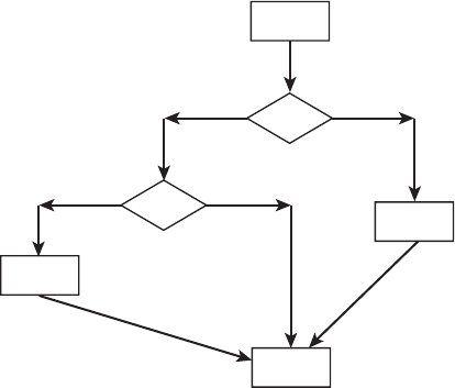
Let’s look at a simple example of the flow diagram shown in Figure 8.1. This diagram
has seven edges (e1 through e7) and six nodes (n1 through n6). Thus McCabe’s cyclo-
matic complexity equals 7 edges 2 6 nodes + 2 = 3. Utilizing the closed region approach,
we have two regions (Region 1 and Region 2) and the cyclomatic complexity equals 2
regions + 1 = 3. The easiest approach may be to count the number of binary decisions
or branches. In this case, there are two (n2 and n4). The cyclomatic complexity number
equals 2 branches + 1 = 3.
Figure 8.1 A simple flow diagram for cyclomatic complexity.
n
1
n
2
n
4
n
5
n
6
e
6
e
3
e
2
e
1
e
7
e
5
e
4
n
3
Region 2
Region 1
168 Chapter 8 Design Characteristics and Metrics
91998_CH08_Tsui.indd 168 1/10/13 6:45:28 AM

The cyclomatic complexity measures the structural design complexity within the
program. It has been applied to design and code risk analysis during development as
well as to test planning for assessing the number of test cases needed to test every deci-
sion point in the design or program. A large number of data has been accumulated, and
we now know that the higher the cyclomatic complexity number, the more risk exists
and that more testing is needed. An example of comparing the cyclomatic complex-
ity numbers against a set of relative risk threshold may be obtained from the Software
Engineering Institute (SEI) website. According to SEI, a cyclomatic complexity number in
the range of 1 through 10 may be viewed as low risk and simple while the other extreme
of very high risk is any cyclomatic number greater than 50. Thus, at the program design
level, we should keep the control flow such that the cyclomatic complexity number is
much smaller than 50.
A cyclomatic number is also the maximum number of linearly independent paths
through the flow diagram. A path in the control flow is linearly independent from other
paths only if it contains some edge, or path segment, that has not been covered before.
Thus the cyclomatic complexity number is also often used to determine the number of
test cases needed to drive through the linearly independent paths in the system.
8.2.3 Henry-Kafura Information Flow
The Henry-Kafura metric is another structural metric, but it measures intermodular flow.
It is based on the flow of information in and out of a module. A count is made of all the
information that comes in and goes out of every module. An information flow includes
the following:
n
Parameter passing
n
Global variable access
n
Inputs
n
Outputs
Thus an information flow is a measure of interactions between modules or between a
module and its environment. Based on information flow, Henry and Kafura developed a
metric where fan-in and fan-out represent the following:
n
Fan-in: Number of information flow into a program module
n
Fan-out: Number of information flow out of a program module
The fan-in of a program module, mod-A, is often viewed as a count of number of mod-
ules that call mod-A. Fan-in also includes the number of global data variables accessed
by mod-A. The fan-out of a program module, mod-A, is the number of program modules
called by mod-A and the number of global data variables accessed by mod-A. Based
on these definitions of fan-in and fan-out, the Henry-Kafura structural complexity for a
program module p, C
p
, is defined as the square of the product of fan-in and fan-out as
follows:
C
p
= (fan-in 3 fan-out)
2
8.2 Some Legacy Characterizations of Design Attributes
169
91998_CH08_Tsui.indd 169 1/10/13 6:45:28 AM

Consider an example where there are four program modules with the fan-in and fan-
out numbers shown in Table 8.1.
The C
p
for each of the four program modules, mod-A through mod-D, are computed
as follows:
C
p
for Mod-A = (3 3 1)
2
= 9
C
p
for Mod-B = (4 3 2)
2
= 64
C
p
for Mod-C = (2 3 3)
2
= 36
C
p
for Mod-D = (2 3 2)
2
= 16
The total Henry-Kafura structural complexity for all four program modules would be
the sum of these, which is 125.
The Henry-Kafura measure of design structural complexity was later modified by
Henry and Selig to include the internal complexity of the program module as follows:
HC
p
= C
ip
3 (fan-in 3 fan-out)
2
The C
ip
is the internal complexity of the program module p, which may be measured
by any code metric such as the cyclomatic or the Halstead metrics. Clearly, we believe
that a high Henry-Kafura number means a complex design structure. Whether this
necessarily leads to a less understandable design and low-quality software is not yet
conclusive.
8.2.4 A Higher-Level Complexity Measure
Card and Glass also utilized the concept of fan-in and fan-out to describe the complex-
ity of a design, which also considers the data that are passed. This is a little higher-level
measure in that it is a set of metrics that cover program level and interprogram level
interactions. They define three design complexity measures:
n
Structural complexity
n
Data complexity
n
System complexity
The structural complexity, S
x
, of a module x is defined as follows:
S
x
= (fan-out
x
)
2
Again, fan-out is the number of modules that are directly invoked by module x. The
data complexity, D
x
, is also defined in terms of fan-out.
D
x
= P
x
/ (fan-out
x
+ 1)
Table 8.1 Fan-in and Fan-out by Program Module
Module Mod-A Mod-B Mod-C Mod-D
Fan-in 3 4 2 2
Fan-out 1 2 3 2
170 Chapter 8 Design Characteristics and Metrics
91998_CH08_Tsui.indd 170 1/10/13 6:45:28 AM

P
x
is the number of variables that are passed to and from module x, and the system
complexity, C
x
, a higher-level measure, is defined as the sum of structural and data com-
plexity:
C
x
= S
x
+ D
x
Note that this measure of design, called system complexity, is based mostly on fan-out.
Fan-in is not really included here except for the data that flow into the module.
8.3 “Good” Design Attributes
We all agree that design is an important activity and should be given ample time and
attention so that we can develop a good design. But what are the characteristics of
a good design? Immediately, we can hear ourselves throw out some of the following
popular terms:
n
Easy to understand
n
Easy to change
n
Easy to reuse
n
Easy to test
n
Easy to integrate
n
Easy to code
In our discussions earlier in this chapter describing Halstead, McCabe, Henry-Kafura,
and Card and Glass metrics, we alluded to intramodular and intermodular complexi-
ties as a factor that relates to software quality. Is there some more fundamental way
to characterize a good design besides listing the different “easy to _____” items? They
themselves may not be the characteristics of a good design and are in fact just the
desirable results achieved with a good design. The common thread to all these “easy
to” properties is the notion of simplicity. A large and complex problem may be simpli-
fied via separation and decomposition into smaller pieces that may be solved in an
incremental fashion (as discussed in Chapter 2). Several design techniques also follow
this principle of simplicity (see Chapter 7). According to Yourdon and Constantine
(1979), the notion of simplicity may be measured by two characteristics: cohesion and
coupling. G. J. Myers (1978) and, more recently, Lethbridge and Laganiere (2001) have
also defined these concepts in their books. These two concepts are not far from the
complexity measures mentioned earlier. Cohesion addresses the intramodule charac-
teristics somewhat similar to Halstead and McCabe metrics, and coupling addresses the
intermodule characteristics similar to the Henry-Kafura fan-in and fan-out information
flow measurements and the system complexity measure of Card and Glass. In general,
we are striving for strong cohesion and loose coupling in our design. Both concepts are
explained in more detail in the following sections.
8.3.1 Cohesion
One of the key notions related to the issue of keeping the design simple so that it will
have many of the desirable “easy to” attributes mentioned earlier is to ensure that each
unit of the design, whether it is at the modular level or component level, is focused on
8.3 “Good” Design Attributes
171
91998_CH08_Tsui.indd 171 1/10/13 6:45:28 AM

a single purpose. Terms such as intramodular functional related-
ness or modular strength have been used to address the notion
of design cohesion. This same notion will be later applied to the
object-oriented (OO) paradigm in Section 8.4.
As we can see from our definition of the notion of cohesion,
depending on the paradigm, the elements may be different.
For example, in the structured paradigm, the elements may be I/O logic, control logic,
or database access logic. In the OO paradigm, the elements may be the methods and
the attributes. Whatever the paradigm, in a highly cohesive design unit the pieces of
that design unit are all related in serving a single purpose or a single function. The
term degree is used in the definition of cohesion. This suggests that there is some
scaling of the attribute.
Generally, seven categories of cohesion can be shown to indicate their relative rank-
ing from bad to good:
n
Coincidental
n
Logical
n
Temporal
n
Procedural
n
Communicational
n
Sequential
n
Functional
Note that there is no numerical assignment provided to help the scaling. This is just a
relative ordering of the categories of cohesion.
The lowest level is coincidental cohesion. At this level the unit of design or code is per-
forming multiple unrelated tasks. This lowest level of cohesion does not usually happen
in an initial design. However, when a design experiences multiple changes and modi-
fications, whether through bug fixes or requirements changes, and is under schedule
pressures, the original design can easily erode and become coincidental. For example,
we might be facing a case where, instead of redesigning, a branch is taken around seg-
ments of design that are now not needed or partially needed and new elements are
inserted due to convenience. This will easily result in multiple unrelated elements in a
design unit.
The next level is logical cohesion. The design at this level performs a series of similar
tasks. At first glance, logical cohesion seems to make sense in that the elements are
related. However, the relationship is really quite weak. An example would be an I/O unit
designed to perform all the different reads and writes to the different devices. Although
these are logically related in that they all perform reads and writes, the read and write
design is different for each device type. Thus at the logical cohesion level, the elements
put together into a single unit are related but are still relatively independent of each
other.
Design at the temporal cohesion level puts together a series of elements that are related
by time. An example would be a design that combines all the data initialization into one
unit and performs all the initialization at the same time even though the data may be
defined and utilized in other design units.
Cohesion An attribute of a unit of high- or
detail-level design that identifies the degree
to which the elements within that unit
belong or are related together.
172 Chapter 8 Design Characteristics and Metrics
91998_CH08_Tsui.indd 172 1/10/13 6:45:28 AM

The next highest level is procedural cohesion. This involves actions that are procedur-
ally related, which means that they are related in terms of some control sequence. This is
clearly a design that shows a tighter relationship than the previous one.
Communicational cohesion is a level at which the design is related by the sequence
of activities, much like procedural cohesion, and the activities are targeted on the same
data or the same sets of data. Thus, designs at the communicational cohesion level dem-
onstrate even more internal closeness than those at the procedural cohesion level.
The last two levels, sequential and functional cohesion, are the top levels where the
design unit performs one main activity or achieves one goal. The difference is that at the
sequential cohesion level the delineation of a “single” activity is not as clear as the func-
tional cohesion level. It is not totally clear that having a design unit at a functional cohe-
sion level is always achievable. Clearly, a design unit at this level, being single-goal ori-
ented, would require very few changes for reuse if there is a need for a design to achieve
the same goal. The sequential cohesion level may still include some elements that are not
single-goal oriented and would require some modifications for reuse.
These levels are not always clear cut. They may be viewed as a spectrum of levels that
a designer should try to achieve as high a level as possible. In design, we would strive
for strong cohesion. Although this approach to viewing cohesion is a good guideline, an
example of a more tangible and quantitative measure of cohesion is introduced next.
Program Slice- and Data Slice-Based Cohesion Measure Bieman and Ott (1994)
introduced several quantitative measures of cohesion at the program level based on
program and data slices. We will briefly summarize their approach to measuring cohe-
sion. First, several definitions will be given, and then an example will follow. Consider a
source program that includes variable declarations and executable logic statements as
the context. The following concepts should be kept in mind:
n
A data token is any variable or constant.
n
A slice within the program or procedure is all the statements
that can affect the value of some specific variable of interest.
n
A data slice is all the data tokens in a slice that will affect the
value of a specific variable of interest.
n
Glue tokens are the data tokens in the procedure or program
that lie in more than one data slice.
n
Superglue tokens are the data tokens in the procedure or pro-
gram that lie in every data slice in the program.
From these basic definitions, it is clear that glue tokens and
superglue tokens are those that go across the slices and offer the
binding force or strength of cohesion. Thus, when quantitatively evaluating the program
cohesion, we would be counting the number of these glue and superglue tokens. More
specifically, Bieman and Ott (1994) define the following two measures for measuring
functional cohesion.
Weak functional cohesion = Number of glue tokens / Total number of data tokens
Strong functional cohesion = Number of superglue tokens / Total number of data
tokens
Data token Any variable or constant.
Program or procedure slice All the state-
ments that can affect the value of some
specific variable of interest.
Data slice All the data tokens in a slice
that will affect the value of a specific vari-
able of interest.
Glue tokens The data tokens in the pro-
cedure or program that lie in more than one
data slice.
Superglue tokens The data tokens in the
procedure or program that lie in every data
slice in the program.
8.3 “Good” Design Attributes
173
91998_CH08_Tsui.indd 173 1/10/13 6:45:29 AM

Both weak and strong functional cohesion use the total number of data tokens as the
factor to normalize the measure. An example will clarify some of these concepts.
Figure 8.2 shows a pseudocode example for a procedure that computes both the
maximum value,
max, and the minimum value, min, from an array of integers in z. The
labeling of the data tokens needs a little explanation. The first appearance of a variable,
n,
in the procedure is labeled
n1. The next appearance of the same variable, n, is labeled n2.
There are a total of 33 data tokens in this procedure. The data slice of code slice around
the variable of interest,
max, and the data slice of code slice around the variable of inter-
est,
min, are represented by data slice max and data slice min respectively in Figure 8.2. In
this case, they have the same number—
22—of data tokens because all the code, except
for the initialization of
min and max to z[0] and the if statements, are the same in con-
tributing to the computation of the maximum or the minimum value. For this example,
the glue tokens are also the same as the superglue tokens. The weak and strong cohesion
measures are as follows.
Weak functional cohesion = 11/33
Strong functional cohesion = 11/33
This procedure computes both the maximum and the minimum value of an array,
z,
of numbers. Now, consider pulling out those instructions that contribute to computing
minimum value and focus only on the maximum value. Then the data slice
max, with
22 data tokens, becomes the whole set of data tokens. It would also be the set of glue
Figure 8.2 A pseudocode example of functional cohesion measures.
Data To kens:
z1
n1
end1
min1
max1
I1
end2
n2
max2
z2
01
min2
z3
02
I2
03
I3
end3
I4
z4
I5
max3
max4
z5
I6
z6
I7
min3
min4
z7
I8
max5
min5 (33)
z1
n1
end1
max1
I1
end2
n2
max2
z2
01
I2
03
I3
end3
I4
z4
I5
max3
max4
z5
I6
max5
(22)
z1
n1
end1
min1
I1
end2
n2
min2
z3
02
I2
03
I3
end3
I4
z6
I7
min3
min4
z7
I8
min5
(22)
z1
n1
end1
I1
end2
n2
I2
03
I3
end3
I4 (11)
z1
n1
end1
I1
end2
n2
I2
03
I3
end3
I4 (11)
Slice max: Slice min: Superglue:Glue To kens:
Finding the maximum and
minimum values
procedure
MinMax (z, n)
integer end, min, max, i;
end = n,
max = z[0];
min = z[0];
For (i = 0, i = < end; i++){
if z[i] > max then max = z[i];
if z[i] > min then max = z[i];
}
return max, min;
174 Chapter 8 Design Characteristics and Metrics
91998_CH08_Tsui.indd 174 1/10/13 6:45:29 AM

tokens and the set of superglue tokens. The functional cohesion measures become as
follows:
Weak functional cohesion = 22/22
Strong functional cohesion = 22/22
By focusing on only one function, maximum value, the cohesion measures have
improved from 11/33 to 22/22. Although this example uses actual code, the concept of
strong cohesion is well demonstrated.
8.3.2 Coupling
In the previous section we focused on cohesion within a software unit. Again, the
term software unit may be a module or a class. Assuming that we are successful in
designing highly cohesive software units in a system, it is most
likely that these units would still need to interact through the
process of coupling. The more complicated the interaction is,
the less likely that we will achieve the “easy to” characteristics
mentioned in the beginning of Section 8.3. A good example of
why analysis of coupling is important is provided by Gamma et al. (1995), who state
that tightly coupled classes are hard to reuse in isolation. That is, a class or a module
that is highly dependent on other modules or classes would be very difficult to under-
stand by itself. Thus it would be difficult to reuse, modify, or fix that module or class
without understanding all the dependent modules and classes. Also, if there is an
error in a module or class that is highly interdependent and is tightly connected with
other modules or classes, then the probability of an error in one affecting the others
is greatly increased. Thus we can see that high coupling is not a desirable design attri-
bute. Several research studies have shown the coupling attribute to be closely associ-
ated with factors such as proneness to error, maintainability, and testability of soft-
ware; see Basili, Briand, and Melo (1996) and Wilkie and Kitchenham (2000) for more
on these relationships.
Coupling is defined as an attribute that specifies the interdependence between two
software units. The amount or degree of coupling is generally divided into five distinct
levels, listed from the worst to the best:
n
Content coupling
n
Common coupling
n
Control coupling
n
Stamp coupling
n
Data coupling
Content coupling is considered the worst coupling and data coupling is considered
to be the best coupling. What is not listed is the ideal situation of no coupling. Of course,
not many problems are so simple that the solutions do not require some coupling. The
common terminology used to describe heavy interdependence and light interdepen-
dence is tight coupling and loose coupling, respectively.
Coupling An attribute that addresses the
degree of interaction and interdependence
between two software units.
8.3 “Good” Design Attributes
175
91998_CH08_Tsui.indd 175 1/10/13 6:45:29 AM

Content coupling between two software units is the worst level. It is considered the
tightest level of coupling because at this level two units access each other’s internal data
or procedural information. In this situation, almost any change to one unit will require a
very careful review of the other, which means that the chance of creating an error in the
other unit is very high. The two units would almost have to be considered as a pair for
any type of reuse of software component.
Two software units are considered to be at the common-coupling level if they both
refer to the same global variable. Such a variable may be used for various information
exchanges, including controlling the logic of the other unit. It is not uncommon to
see common coupling exhibited in large commercial applications where a record in
the database may be used as a global variable. Common coupling is much better than
content coupling. It still exhibits a fairly tight amount of coupling because of the per-
meating effects a change to the global variable or the shared database record would
have on those that share this variable or record. In large application developments, the
“where-used” matrix is generated during the system-build cycle to keep track of all the
modules, global variables, and data records that are cross-referenced by the different
software units. The where-used matrix is extensively used by both the integration team
and the test team.
Control coupling is the next level where one software unit passes a control infor-
mation and explicitly influences the logic of another software unit. The data that have
been passed contain embedded control information that influences the behavior of
the receiving software unit. The implicit semantics codified in the passed information
between the sending and receiving modules force us to consider both modules as a
pair. This level of coupling binds the two software units in such a manner that a single
software unit reuse, separate from the others, is often hindered. Testing is also further
complicated in that the number of test cases for interunit dependencies may increase
dramatically when the embedded control information is deeply encoded.
In stamp coupling, a software unit passes a group of data to another software unit.
Stamp coupling may be viewed as a lesser version of data coupling in that more than
necessary data are passed between the two software units. An example would be pass-
ing a whole record or a whole data structure rather than only the needed, individual
datum. Passing more information certainly increases the difficulty of comprehending
what the precise interdependence between the two software units is.
The best level of coupling is data coupling, where only the needed data are passed
between software units. At the data-coupling level, the interdependence is low and the
two software units are considered loosely coupled.
These coupling levels do not include every possible interdependence situation. For
example, a plain invocation of another software unit with only a passing of control and
not even requiring a return of control is not mentioned. There is also no distinction made
between data passed from one software unit to another, which may include the return of
data where the returning information would be at a different coupling level. We should
view the levels of coupling, like the levels of cohesion, as a guideline for good design.
That is, we should strive for simplicity via strong cohesion and loose coupling in our
design and coding.
176 Chapter 8 Design Characteristics and Metrics
91998_CH08_Tsui.indd 176 1/10/13 6:45:29 AM

Fenton and Melton (1990) provided a relatively simple example of measuring cou-
pling between two software units, x and y, as follows:
1. Assign each level of coupling, from data coupling to content coupling, a numerical
integer from 1 through 5, respectively.
2. Evaluate software units x and y by identifying the highest or the tightest level of
coupling relationship between the x, y pair and assign it as i.
3. Identify all the coupling relationships between the pair x and y, and assign it as n.
4. Define the pairwise coupling between x and y as C(x, y) = i + [n/(n + 1)].
For example, x passes y specific data that contain embedded control information
that will influence the logic of y. Also x and y share a global variable. In this case, there
are two coupling relationships between x and y. So n = 2. Of the two relationships,
common coupling is worse, or tighter, than control coupling. So the highest coupling
level between x and y is 4, which is common coupling. Thus i = 4, which then means
that C(x, y) = 4 + [2 /(2 + 1)]. With this definition, the smaller the values of i and n are,
the looser the coupling will be. If all the software units in a system are pairwise analyzed
as this, we can get a feel for the overall software system coupling. In fact, Fenton and
Melton (1990) define the overall global coupling of a system to be the median value of
all the pairs. Thus, if a software system, S, included x
1
, . . ., x
j
units, then C(S) = median of
the set {C(x
n
, x
m
), for all the n, m from 1 through j }. Thus, we would want to strive toward
a lower C(S) when designing a software system.
8.4 Object-Oriented Design Metrics
In this section we explore how the earlier notion of keeping the design simple through
decomposition, strong cohesion, and loose coupling is affected, if any, by the object-
oriented design and programming paradigm. Although there are several important
concepts in OO, including class, inheritance, encapsulation, and polymorphism, there is
really one central theme. That theme involves classes, how these classes are interrelated
to each other, and how the classes interact with each other. A class is just a software
entity that we want to, once again, keep simple through strong cohesion. The inter-
relationship and interaction among the classes should be kept simple through loose
coupling. Thus the good, desirable design attributes have not changed. In OO, there are,
however, some extensions to the way we would measure these attributes.
The desirable attributes of a good OO design may be measured by the six C-K metrics,
which were identified by Chidamber and Kemerer (1994):
1. Weighted methods per class (WMC)
2. Depth of inheritance tree (DIT)
3. Number of children (NOC)
4. Coupling between object classes (CBO)
5. Response for a class (RFC)
6. Lack of cohesion in methods (LCOM)
8.4 Object-Oriented Design Metrics
177
91998_CH08_Tsui.indd 177 1/10/13 6:45:29 AM

Studies by Basili, Briand, and Melo (1996), Li and Henry (1993), and Briand et al. (2000)
have shown that these (C-K) metrics correlate and serve well as indicators of error prone-
ness, maintainability, and so on.
WMC is a weighted sum of all the methods in a class. Thus if there are n methods,
m
1
through m
n
, in a class, then WMC = SUM(w
i
), where i = 1, . . ., n. SUM is the arithmetic
summation function, and w
i
is the weight assigned to method m
i
. A simple situation is
to just count the number of methods by uniformly assigning 1 as the weight for all the
methods. So a class with n methods will have its WMC equal to n. This metric is similar
to counting the lines of code, where we find that the larger the size of the module, the
more likely it will be prone to error. Larger classes, particularly those with larger WMCs,
are associated with more error-proneness.
DIT is the maximum length of inheritance from a given class to its “root” class. It seems
that the chance of error increases as we engage in inheritance and multiple inheritances.
It is interesting to note that in the early days of OO, many organizations ignored inheri-
tance features, designed their own unique classes, and never realized the desired pro-
ductivity gain from reuse or inheritance. They thought it was simpler to design their own
classes and not have to fully understand other, predefined classes. A class placed deep
in the inheritance hierarchy was also difficult to even find, let alone fully comprehend.
However, the various empirical tests have shown mixed results. Some have shown large
DIT is associated with high defect rates, and others have found results inconclusive.
The NOC of a class is the number of children, or its immediate subclasses. This OO metric
has also had mixed empirical results. When the NOC of all the classes are added together,
it would seem that a large NOC of the software system could influence the complexity of
the system. At the writing of this book, it is still uncertain how NOC influences the quality
of the software.
CBO represents the number of object classes to which it is coupled. This is intuitively
the same as the traditional coupling concept. Tighter or more coupling among classes
where they share some common services or where one inherits methods and variables
from other classes certainly introduces complexity, error-proneness, and difficulty of
maintenance.
RFC is the set of methods that will be involved in a response to a message to an object
of this class. RFC is also related to the notion of coupling. It has been shown that this
metric is highly correlated to CBO and WMC. Because both large CBO and large WMC
are known to affect defects and complexity of the software system, large RFC is also cor-
related with high defects.
LCOM is a count of the difference between the method pairs that are not similar and
those that are similar within a given class. This metric characterizes the lack of cohesion
of a class. It requires a bit more explanation and an example:
Consider a class with the following characteristics:
n
It has m
1
, . . ., m
n
methods.
n
The instance variables or attributes in each method are represented as I
1
, . . ., I
n
, respec-
tively.
Let P be the set of all the method pairs that have noncommon instance variables, and
let Q be the set of all the method pairs that have common instance variables. Then LCOM =
#P 2 #Q, where # represents cardinality of the set. Thus we can see that a class with a high
178 Chapter 8 Design Characteristics and Metrics
91998_CH08_Tsui.indd 178 1/10/13 6:45:29 AM

LCOM value indicates that there is a high number of disparate methods. Therefore classes
with high LCOM values are less cohesive and may be more complex and difficult to under-
stand. High LCOM value equates with weak cohesion. To properly complete the definition
of this metric, it must be stated that if #P is not > #Q, then LCOM = 0.
For example, a class, C, may contain three methods (m
1
, m
2
, m
3
) whose respective
instance variable sets are I
1
= {a, b, c, s}, I
2
= {a, b, z}, and I
3
= {f, h, w}. The I
1
and I
2
have {a,
b} in common. I
1
and I
3
have nothing in common, and I
2
and I
3
also have nothing in com-
mon. In this case, #P, the number of method pairs that are not similar or have nothing in
common, is 2. The number of method pairs that are similar or have something in com-
mon, #Q, is 1. Thus LCOM for class C = 2 2 1 or 1.
All of these six C-K design metrics, are related either directly or indirectly to the
concepts of cohesion and coupling. These metrics should assist software designers in
better understanding the complexity of their design and help direct them to simplify-
ing their work. As Figure 8.3 shows, what the designers should strive for is strong
cohesion and loose coupling.
8.4.1 Aspect-Oriented Programming
Aspect-oriented programming (AOP) is a new evolution of the concept for the separation of
concerns, or aspects, of a system. This approach is meant to provide more modular, cohe-
sive, and well-defined interfaces or coupling in the design of a system. Central to AOP is the
notion of concerns that cross cut, which means that the methods related to the concerns
intersect. It is believed that in OO programming these cross-cutting concerns are spread
across the system. Aspect-oriented programming would modularize the implementation
of these cross-cutting concerns into a cohesive single unit. Kiczales et al. (1997), Elrad,
Filman and Bader (2001), and Colyer and Clement (2005) provide more information on
aspect-oriented programming.
8.4.2 The Law of Demeter
Another good guideline for object-oriented design is the Law of Demeter, addressed by
Lieberherr and Holland (1989). This guideline limits the span of control of an object by
Figure 8.3 Cohesion and coupling.
Strong
Weak Loose
Tight
High level
Low level
Cohesion
Coupling
8.4 Object-Oriented Design Metrics
179
91998_CH08_Tsui.indd 179 1/10/13 6:45:29 AM

restricting the message-sending structure of methods in a class. The messaging restric-
tion will reduce the coupling of objects and enhance the cohesion of an object. This is
not a measurement but a guideline originating from the experience gained from the
design and implementation of the Demeter System, an aspect-oriented programming
project at Northeastern University, developed in the 1980s.
The Law of Demeter may be stated as follows. An object should send messages to the
following kinds of objects:
n
The object itself
n
The object’s attributes (instance variables)
n
The parameters of methods in this object
n
Any object created by the methods of this object
n
Any object returned from a call to one of this object’s methods
n
Any object in any collection that is one of the preceding categories
The law essentially ensures that objects send messages only to objects that are
directly known to them. It may be paraphrased as “only talk to your immediate neigh-
bors” or “don’t talk to strangers.” A simple example, adapted from management control,
may help. Consider the case of a software development vice president who wishes to
enforce a design principle across the development organization. Rather than giving the
command to his or her immediate subordinates and asking them, in turn, to relay the
message to their subordinates, the vice president engages in direct conversation with
every person in the organization. Clearly such an approach increases coupling and dif-
fuses cohesion. This vice president has violated the Law of Demeter.
8.5 User-Interface Design
Up until now, we have focused on software units and the interactions among them. In
this section we will concentrate on user-interface (UI) design—the interactions between
a human user and the software. Instead of worrying about reducing software defects, we
must now worry about reducing human errors. Although some designers may believe
that having a graphical user interface solves many of the user anxiety problems with
computing systems, it is still important to understand what is it that makes the interface
easier to understand, navigate, and use. What is user-friendliness, and what characterizes
a good user-interface design? The important characteristic here is that the interface has
more to do with people rather than software systems.
8.5.1 Good UI Characteristics
In Section 8.1, we listed consistency and completeness as two general design character-
istics. In UI design, consistency is especially important because it contributes to many
of the desirable characteristics that a human requires. Imagine a user interface that has
inconsistent headings or labels, inconsistent help texts, inconsistent messages, inconsis-
tent response times, inconsistent usage of icons, or inconsistent navigation mechanisms.
Imagine an even worse situation where some of the inconsistencies lead to an actual
conflict that a user is pressed to resolve; see Nielson (2002) for additional discussion of
UI consistency.
180 Chapter 8 Design Characteristics and Metrics
91998_CH08_Tsui.indd 180 1/10/13 6:45:29 AM

One of the main goals for UI design is to ensure that there is a consistent pattern across
all the interfaces. Mandel (1997) has identified three “golden rules” for user-interface
design:
n
Place the user in control
n
Reduce the user’s memory load
n
Design consistent user interface
These rules have further spawned another two principles for UI design: (1) user action
should be interruptible and allowed to be redone, and (2) user defaults should be mean-
ingful. These rules and principles all serve as good guidelines for UI design.
Shneiderman and Plaisant (2005) have identified the following eight rules of interface
design:
1. Strive for consistency
2. Enable frequent users to use short cuts
3. Offer informative feedback
4. Design dialogues to yield closure
5. Offer error prevention and simple error handling
6. Permit easy reversal of actions
7. Support internal locus of control
8. Reduce short-term memory
Note that consistency, which we have already discussed, is the first on the list. The sec-
ond rule, which involves short cuts to achieve an end goal, indicates that there may need
to be different levels of user interface for novices and for experts. The feedback from the
system to the user should be informative and understandable so that the user will know
what follow-up action to perform, if any. The user activities should be grouped in such
a manner that there is a start and an end; the user should experience a sense of accom-
plishment at the end of the series of activities. The fifth and sixth rules deal with human
fallibility. The system should be designed to prevent the user from making mistakes. But if
an error is made, there needs to be a mechanism that allows the user to reverse or handle
the mistake. The seventh rule addresses the human need for control. That is, the users
should not be made to respond to the software system; instead, the system should be
made to respond to user-initiated actions. The eighth rule recognizes the limitations of
human memory and that information should be kept simple. Wherever possible, informa-
tion should be provided to the users in the form of defaults or in the form of preassigned
lists of choices. This theory on short-term memory is often attributed to Miller (1956), who
identified “seven, plus or minus two” limits on our ability to process information.
In addition to the preceding rules, there are also various UI guideline standards.
Large corporations such as IBM, Microsoft, and Apple have their own UI guidelines. The
International Standards Organization (ISO) has several standards related to user inter-
faces, including ISO 9241, which has multiple parts that can be acquired from the ISO
website at www.iso.org.
8.5.2 Usability Evaluation and Testing
In the 1980s, with the advent of personal computers and graphical interface, UI designs
received a lot of attention. Usability testing became a new task that was introduced
8.5 User-Interface Design
181
91998_CH08_Tsui.indd 181 1/10/13 6:45:29 AM

into software development. In its early state, the UI design was of low fidelity in that
the interfaces were mocked-up with paper boards and diagrams. As the technology
and tools improved, UI design became high fidelity in that real screens were developed
as design prototypes. Some of these prototypes were introduced during the require-
ments phase. With the high-fidelity UI design, more in-depth evaluation was performed.
Elaborate usability “laboratories” with one-way mirrors and recording equipment were
constructed, and statistical analysis of user performance was conducted. Users, or sub-
jects, were carefully profiled and chosen for the usability tests.
Some of the key factors in analyzing application interfaces included the following:
n
Number of subjects who completed the tasks without any help
n
Length of time, on the average, required to complete each task
n
Average number of times that help function was evoked
n
Number of tasks completed within some predefined time interval
n
Places where subjects had to redo a task, and the number of times this needed to be
done
n
Number of times short cuts were used
These and other types of information were recorded and analyzed. Sometimes there
was also a questionnaire that would further ask for the subjects’ comments on the gen-
eral appearance, flow, or suggestions.
In the early days of usability testing, this activity was grouped as a type of postsystem
testing and was conducted late in the development cycle. As a result of placing usability
testing late in the testing cycle, only the most severe problems were fixed. The other,
lesser problems were all delayed and assigned to the next release. Today, UI evaluation
is moved up to the requirements and design phases. Many of the problems are resolved
early, and the solutions are integrated into the software product in time for the current
product release.
8.6 Summary
In this chapter, we first introduced two general characteristics of a good design:
n
Consistency
n
Completeness
A list of early concepts related to design complexity and metrics were then intro-
duced.
n
Halstead complexity measure
n
McCabe’s cyclomatic complexity
n
Henry-Kafura flow complexity measure
n
Card and Glass structural complexity measure
The two main criteria for a simple and good design that can provide us the various
“easy to” attributes are discussed in detail. The goal is to attain the following:
n
Strong cohesion
n
Weak coupling
182 Chapter 8 Design Characteristics and Metrics
91998_CH08_Tsui.indd 182 1/10/13 6:45:29 AM
A specific example, using techniques from Bieman and Ott (1994), is also shown to
clarify the notion of cohesion.
The six C-K metrics for OO design are shown to be also closely tied to the notion of
cohesion and coupling:
n
Weighted methods per class (WMC)
n
Depth of the inheritance tree (DIT)
n
Number of children (NOC)
n
Coupling between object classes (CBO)
n
Response for a class (RFC)
n
Lack of cohesion in methods (LCOM)
Finally, with the advent of graphical interface and the Internet, the characteristics of
good user-interface design are discussed. UI design should focus on the human rather
than on the system side. In today’s systems, much of the late usability testing is moved
up into UI interface prototyping conducted during the early requirements phase.
8.7 Review Questions
1. What are the two general characteristics of a good design that naturally evolve
from requirements?
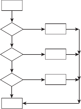
2. What is the cyclomatic complexity of the design flow shown in Figure 8.4 where
the diamond shapes represent decision branches and the rectangles are state-
ments?
3. What are glue tokens and superglue tokens? Which contributes more to cohesion
and why?
4. What are the levels of cohesion?
Figure 8.4 Case structure.
s2
s1
C1
s5
s3
C2
s4
C3
8.7 Review Questions
183
91998_CH08_Tsui.indd 183 1/10/13 6:45:29 AM

5. What are the levels of coupling?
6. What are the six C-K metric for OO design?
7. What is a depth of inheritance tree (DIT) in C-K metrics, and why may a large DIT
be bad for design?
8. In contrast to general design, what is of the most interest in user-interface design?
9. List four of the eight rules of interface design presented by Shneiderman and
Plaisant.
8.8 Exercises
1. Discuss the difference between a good design and what we are trying to achieve
as a result of a good design.
2. In gauging design, one of the concepts involves fan-in and fan-out.
a. Discuss the concept of fan-in and fan-out in a design.
b. In Henry-Kafura’s measure, complexity is defined as C
p
, where C
p
= (fan-in 3
fan-out)
2
. Instead of multiplying fan-in and fan-out, discuss the effect if you
change the operator to addition, especially for the situation when the number
of fan-in or fan-out values increases.
3. Why do you suppose Card and Glass focused more on the fan-out value rather
than on the number of fan-ins?
4. Define cohesion in your own words.
5. Define coupling in your own words.
6. The notion of an entity relationship (ER) diagram was evolved into a database
design, as discussed in Chapter 7. If various components use the same database
table to update records and query records, what type of coupling is involved?
Explain.
7. Is there any conflict between strong cohesion and weak coupling? Discuss.
8. Does the cyclomatic measure have anything to do with the concept of cohesion
or coupling? Explain how it does or does not.
9. Summarize one of Mandel’s UI golden rules. Place user in control, subject to some
of Shneiderman and Plaisant’s UI golden rules, and discuss why you chose those.
10. Relate one of the UI golden rules, reduce user’s memory load, to other design
characteristics such as simplicity in design, strong cohesion, and weak coupling.
8.9 Suggested Readings
E. Arisholm, L. C. Briand, and A. Foyen, “Dynamic Coupling Measurement for Object-
Oriented Software,” IEEE Transactions on Software Engineering 30, no. 8 (August 2004):
491–506.
184 Chapter 8 Design Characteristics and Metrics
91998_CH08_Tsui.indd 184 1/10/13 6:45:30 AM

V. R. Basili, L. C. Briand, and W. L. Melo, “A Validation of Object-Oriented Design Metrics as
Quality Indicators,” IEEE Transactions on Software Engineering 22, no. 10 (October 1996):
751–761.
J. M. Bieman and L. M. Ott, “Measuring Functional Cohesion,” IEEE Transactions on Soft-
ware Engineering 20, no. 8 (August 1994): 644–657.
L. C. Briand, J. W. Daly, and J. Wust, “A Unified Framework for Cohesion Measurement in
Object-Oriented Systems,” Proceedings of the Fourth International Software Metrics Sympo-
sium (November 1997): pp. 43–53.
L. C. Briand, J. Wüst, J. W. Daly, and D. V. Porter, “Exploring the Relationship Between De-
sign Measures and Software Quality in Object-Oriented Systems,” Journal of Systems and
Software 51, no. 3 (2000): 245–273.
D. N. Card and R. L. Glass, Measuring Software Design Quality (Upper Saddle River, NJ: Pren-
tice Hall, 1990).
S. Chidamber, D. P. Darcy, and C. Kemerer, “Managerial Use of Metrics for Object-Oriented
Software: An Exploratory Analysis,” IEEE Transactions on Software Engineering 24, no. 8
(August 1998): 629–639.
S. Chidamber and C. Kemerer, “A Metrics Suite for Object-Oriented Design,” IEEE Transac-
tions on Software Engineering 20, no. 6 (June 1994): 476–493.
A. Colyer and A. Clement, Aspect-Oriented Programming with AspectJ,” IBM Systems Jour-
nal 44, no. 2 (2005): 302–308.
T. Elrad, R. E. Filman, and A. Bader, “Aspect-Oriented Programming,” Communications of
the ACM (October 2001): 29–32.
K. E. Emam et al., “The Optimal Class Size for Object-Oriented Software,” IEEE Transactions
on Software Engineering 28, no. 5 (May 2002): 494–509.
N. Fenton and A. Melton, “Deriving Structurally Based Software Measure,” Journal of Sys-
tems and Software 12, no. 3 (July 1990): 177–187.
E. Gamma, R. Helm, R. Johnson, and J. Vlissides, Design Patterns: Elements of Reusable
Object-Oriented Software (Reading, MA: Addison-Wesley, 1995).
M. H. Halstead, Elements of Software Science (New York: Elsevier, 1977).
S. M. Henry and D. Kafura, “Software Structure Metrics Based on Information Flow,” IEEE
Transactions on Software Engineering 7, no. 5 (September 1981): 510–518.
S. Henry and C. Selig, “Predicting Source-Code Complexity at Design Stage,” IEEE Software
(March 1990): 36–44.
D. Hix and H. R. Hartson, Developing User Interface: Ensuring Usability Through Product and
Process (New York: Wiley, 1993).
G. Kiczales et al., “Aspect Oriented Programming,” Proceedings of the 11th European Con-
ference on Objected Oriented Computing (June 1997): 220–242.
S. Lauesen, User Interface Design: A Software Engineering Perspective (Reading, MA: Addi-
son-Wesley, 2004).
8.9 Suggested Readings
185
91998_CH08_Tsui.indd 185 1/10/13 6:45:30 AM

T. Lethbridge and R. Laganiere, Object-Oriented Software Engineering: Practical Software
Development Using UML and Java (New York: McGraw-Hill, 2001).
W. Li and S. Henry, “Object-Oriented Metrics That Predict Maintainability,” Journal of Sys-
tems and Software 23 (1993): 111–122.
K. J. Lieberherr and I. Holland, “Assuring good styles for object-oriented programs,” IEEE
Software (September 1989): 38–48.
M. Lorenz and J. Kidd, Object-Oriented Software Metrics: A Practical Guide (Upper Saddle
River, NJ: Prentice Hall, 1994).
T. Mandel, The Elements of User Interface Design (New York: Wiley, 1997).
T. J. McCabe, “A Complexity Measure,” IEEE Transactions on Software Engineering 2, no. 4
(December 1976): 308–320.
T. J. McCabe and B. W. Charles, “Design Complexity Measurement and Testing,” Commu-
nications of the ACM 32, no. 12 (December 1989): 1415–1425.
G. Miller, “The Magical Number Seven, Plus or Minus Two: Some Limits on Our Capacity
for Processing Information,” Psychology Review 63 (1956): 81–97.
G. J. Myers, Reliable Software Through Composite Design (New York: Petrocelli/Charter,
1975).
——, Composite/Structured Design (New York: Nostrand Reinhold, 1978).
J. Nielson, Coordinating User Interfaces for Consistency (New York, NY: Academic Press,
1989; reprint by Morgan Kaufman Publishers, 2002).
——, Designing Web Usability: The Practice of Simplicity (Thousand Oaks, CA: New Riders
Publishing, 2000).
——, http://www.useit.com, 2012.
A. J. Offutt, M. J. Harrold, and P. Kolte, “A Software Metric System for Module Coupling,”
Journal of Systems and Software 20, no. 3 (March 1993): 295–308.
B. Shneiderman and C. Plaisant, Designing the User Interface: Strategies for Effective Human-
Computer Interaction, 4th ed. (Reading, MA: Addison-Wesley, 2005).
R. Subramanyam and M. S. Krishnan, “Empirical Analysis of CK Metrics for Object-Oriented
Design Complexity: Implications for Software Defects,” IEEE Transactions on Software En-
gineering 29, no. 4 (April 2003): 297–310.
F. Tsui, O. Karam, S. Duggins, and C. Bonja, “On Inter-Method and Intra-Method Object-
Oriented Class Cohesion,” International Journal of Information Technologies and Systems
Approach 2(1), (June 2009): 15–32.
F. G. Wilkie and B. A. Kitchenham, “Coupling Measures and Change Ripples in C++ Appli-
cation Software,” Journal of Systems and Software 52 (2000): 157–164.
E. Yourdon and L. Constantine, Structured Design: Fundamentals of a Discipline of Com-
puter Program and Systems Design (Upper Saddle River, NJ: Prentice Hall, 1979).
186 Chapter 8 Design Characteristics and Metrics
91998_CH08_Tsui.indd 186 1/10/13 6:45:30 AM
..................Content has been hidden....................
You can't read the all page of ebook, please click here login for view all page.