

OBJECTIVES
265
CHAPTER
13
Software Project
Management
n
Analyze the four phases of project management:
n
Planning
n
Organizing
n
Monitoring
n
Adjusting
n
Discuss three specific project effort estimating techniques:
n
COCOMO
n
Function point
n
A simple technique for object-oriented environment
n
Describe two more techniques of project management:
n
Work breakdown structure for task scheduling
n
Earned value management for project monitoring
91998_CH13_Tsui.indd 265 1/5/13 10:01:58 AM

13.1 The Necessity of Project Management
We have spent several chapters of this text discussing software design and the software
development process and methodologies. Why can’t we just follow these processes and
methodologies and complete a project? What if a project requires only two or three people?
On the surface it may seem that a small project can just follow a development process
and be left alone to complete a project without any project management. However, we
may question how it is determined that a project needs only two or three people. Is there
a software development process that these people all agree on and have experience in?
Furthermore, how does anyone, including the project team members, know if a project is
progressing properly unless someone is monitoring it?
Even small and fairly simple software projects need project management. What differs
among the various software projects is in the degree of management efforts. A large and
complex software project would require some sophisticated project management skills
and considerable effort, along with tools to aid the management tasks. The key is to strike
a balance between lean project management and excessive project management, never
letting it become too meager or too overbearing.
13.2 The Project Management Process
Many software engineering students, as well as some professionals, confuse software
project management with the software engineering process and development life cycle.
Software project management follows a management process to ensure that the appro-
priate software engineering process is implemented, but it is not itself a software engi-
neering process. Figure 13.1 depicts the high-level flow of a software project manage-
ment process and the four major sets of activities (known as POMA) that are involved:
1. Planning
2. Organizing
3. Monitoring
4. Adjusting
Figure 13.1 Software project management process.
Project
Planning
Project
Organizing
Project
Adjusting
Project
Monitoring
266 Chapter 13 Software Project Management
91998_CH13_Tsui.indd 266 1/5/13 10:01:58 AM

These four activities of POMA may sometimes overlap. Most of the major portions of
the activities are performed in sequence, a flow depicted by the large arrows in the fig-
ure. The curved arrows in Figure 13.1 show how the monitoring and adjustment phases
of project management not only overlap but heavily interact in a cyclic fashion. As the
project status information is gathered and reported, it is often necessary to adjust and
make changes to the project. The combination of monitoring and making the proper
adjustments is what dictates proper project control.
The dashed arrows in Figure 13.1 depict that the needed adjustments may affect
some of the previously set plans, methodologies, organizational policies, reporting struc-
tures, and so on, that were established in earlier phases. While the four POMA phases
appear to be in sequence, there will be incidents in each phase that may cause what was
completed in a previous phase to be altered. Software project management, like other
project management, often requires an iterative process. Tsui (2004) provides additional
information on managing software projects and the concept of POMA.
Project management ensures that the following goals are met:
n
The end results satisfy the customer’s needs.
n
All the desired product/project attributes (quality, security, productivity, cost, etc.) are
met.
n
Target milestones are met along the way.
n
Team members are operating effectively and with high morale.
n
Required tools and other resources are available and effectively utilized.
It is important to remember that a project manager cannot do this alone but has to work
through the team members to accomplish these management targets.
13.2.1 Planning
Planning is a natural first phase of any project. The success and failure of the project rides
heavily on the results of proper planning. Yet so many software projects tend to rush
and minimize this phase citing schedule and cost constraints. Even with a well-planned
project, it is not unusual to still see many changes and modifications. Some will use this
reason to develop a poor plan or even totally skip planning. Having a well-conceived and
documented plan, however, will help facilitate the anticipated modifications that often
occur in a software project.
During the early planning phase, the answers to the following questions will contrib-
ute to the formulation of a project plan:
n
What is the nature of the software project, who is sponsoring the project, and who are
the users?
n
What are the needed requirements and what are the desired requirements?
n
What are the deliverables of the project?
n
What are the constraints of the project (schedule, cost, etc.)?
n
What are the known risks of the project?
Notice that these are very close to the same questions asked during the requirements
gathering and analysis activities. Software engineering’s requirements methodolo-
gies and process provide the directions on how to perform information gathering and
analysis. Project management must ensure that there are qualified resources, proven
13.2 The Project Management Process
267
91998_CH13_Tsui.indd 267 1/5/13 10:01:58 AM

methodology, and ample time set aside to perform the tasks related to answering these
questions. The problem of who funds this part of the planning phase has always been
a difficult business question. Sometimes customers and users are asked to fund these
activities separately; other times the software project organization will sponsor the activ-
ities as costs of doing business and fold them into the cost of the total project. Today,
large, sophisticated organizations realize the importance of this planning phase and are
willing to pay for part of the activities.
Once the basic project requirements are understood, the rest of the project planning
activities are much easier to perform and complete. The following activities are the major
parts of project planning:
n
Ensure that the requirements of the project are accurately understood and specified.
n
Estimate the work effort, the schedule, and the needed resources/cost of the project.
n
Define and establish measurable goals for the project.
n
Determine the project resource allocations of people, process, tools, and facilities.
n
Identify and analyze the project risks.
There are skills and techniques involved in each of these activities. Some will be fur-
ther explained in separate sections of this chapter. Based on the proper completion of
requirements gathering and analysis, the total work effort is estimated. This estimation
is then used to establish a project schedule and cost. The schedule milestones are set
according to the chosen process, tools, skills, and so on.
One of the most difficult tasks during this phase is defining realistic and measurable
goals. We are used to making grand claims about software products—superior quality,
easy to use, easy to maintain. We also like to claim that we have the most efficient and
productive team members or most effective methodology. Unless these claims are well
defined and measurable, they cannot serve as project goals because there will be no way
of monitoring them. As happens in requirements gathering and analysis, a project man-
ager will not be defining these goals alone. It usually is, and should be, a team effort. The
success of a project is determined by whether the jointly planned and agreed to goals
are achieved. Therefore, the project team members should all understand these goals
and measurements. For example, if one of the project goals is to have a high-quality
product, the term high quality must be defined, or no one will know if the goal has been
achieved. But simply defining the term alone is not enough. A common mistake would
be to define high quality as a product that satisfies customer requirements—a definition
that becomes circuitous and useless and does not include and allow quantitative analy-
sis. A goal or definition must be measurable so that as we are monitoring the project we
can ascertain if the product will achieve the high quality expected. The quality goal may
thus be restated more precisely as follows.
The product quality goal is that 98% of the listed functional requirements in
the approved requirements specification document are all tested and have
no known problems at the product release time. The remaining 2% of the
listed functional requirements are also all tested and have no known sever-
ity 1 problems at the product release time. Severity 1 problems are those
that cause the function not be completed and there is no manual work-
around to complete the required function.
268 Chapter 13 Software Project Management
91998_CH13_Tsui.indd 268 1/5/13 10:01:58 AM

Although not perfect, this goal specification provides us with ways to measure the
progress toward the final attainment of a goal. We can quantitatively count the number of
total functional requirements, the number of tested functional requirements, the number
and severity of problems found during the test, and the number and severity of problems
remaining at product release time. With these we can determine whether we have achieved
the quality goal.
Similarly, the goal of meeting project schedule should be stated with more than just
a single date. It must be divided into multiple elements that can be measured along the
way. For example, a schedule goal may be divided into a set of milestone dates and have
a stated goal of meeting 95% of all the milestones along the way as well as meeting the
final completion date. If only the final completion date is stated as the goal, then it would
be very difficult to measure the project’s progress or have any early warning sign of
schedule problems. Very little corrective action can be taken if there is no input on sched-
ule status until the schedule problem has surfaced on the night before the final comple-
tion date. The goals need to be quantitatively measurable and monitored throughout
the project. Nonmeasurable goals are often said to be nonmanageable. The concept of
measurement and metrics is discussed further in a later section of this chapter
Another part of planning activities is the identification and analysis of risk items. There
are very few projects with no risk. Software projects are fraught with cost overruns and
schedule delays. Risk management thus becomes an integral part of software project
management, and all risks must be considered during the planning phase. Risk manage-
ment itself is composed of three major components:
1. Risk identification
2. Risk prioritization
3. Risk mitigation
How do we identify risks? Some fertile areas to look for risks include new methodology,
requirements new to the group, special skills and resource shortage, aggressive schedule,
and tight funding. It is important to consider all possible items that might have a negative
impact on the project. Of course, such a list may be huge and impossible to work with, so
it will be necessary to prioritize the risks and perhaps decide to consider and track only the
high-priority problems. After a prioritized list of risks is agreed on, the planning process
must include an activity set to mitigate these prioritized risks and to take some action.
Hoping that some external force will magically appear and reduce the risks would be fool-
ishly optimistic. A plan to mitigate these risks must thus be included during the project
planning phase.
The activities in a project planning phase all contribute to developing an overall proj-
ect plan. Depending on the projects, some project plans may be quick and short while
others may be very extensive and lengthy. The content of a project plan must include
the following basic items:
n
Brief description of the project requirements and deliverables
n
Set of project estimations
n
Work effort
n
Needed resources
n
Schedule
13.2 The Project Management Process
269
91998_CH13_Tsui.indd 269 1/5/13 10:01:58 AM

n
Set of project goals to be achieved
n
Set of assumptions and risks
The plan may be expanded to include a discussion of the problems to be resolved,
differentiating between those problems that must be fixed and those that it would be
nice to fix. A user and customer profile may be included. A detailed description of all the
major requirements and deliverables may be placed in an appendix portion of the plan.
The work effort estimate may be explained and shown in detail. The required resources
and cost may be broken into major categories of human resources, tools and methodolo-
gies, and facilities. The schedule may be divided into sets of major and minor milestones.
The project goals may be expanded to include multiple project attributes, more than just
meeting schedules and costs. The definition and measurements of all the goals need to
be clearly developed. In addition, a list of assumptions, major risks, and minor risks may
be included. These risks and assumptions may be accompanied with a discussion of how
these risks will be contained throughout the project.
Although it is true that there will always be many unknowns during the planning
stage, the more thorough the project planning phase is, the higher the chance that
project will be successful. This does not mean that there will be no change to the proj-
ect or to the plan. Even the best planned project will face some changes as the earlier
unknowns become clearer. There will also be some justifiable change of heart as the
project progresses. All project managers and project team members should be prepared
for such changes. The authors and proponents of the Agile process discussed in Chapter
5 understand this so well that they plan only for short iterations of development and
caution against excessive planning.
13.2.2 Organizing
Once a project plan has been formulated or even before it has been completed, the
organizing activities must be initiated. For example, as soon as we have the estimated
resources planned, hiring and placement may begin. Table 13.1 shows how some of the
planning and organizing activities may be paired and overlapped.
As soon as a specific planning activity such as risk planning is complete, we can
establish the mechanism for tracking and mitigating the risks. The project manager does
not need to wait for every planning activity to be finished before starting the organizing
phase.
Table 13.1 Pairing Planning And Organizing Activities
Planning Organizing
Project content and deliverables
Project tasks and schedule Set up tracking mechanisms of tasks and schedules
Project resources Acquire, hire, and prepare resources such as people, tools, and processes
Project goals and measurement Establish mechanism to measure and track the goals
Project risks Establish mechanism to list, track, and assign risk mitigation tasks
270 Chapter 13 Software Project Management
91998_CH13_Tsui.indd 270 1/5/13 10:01:58 AM

The organizing phase requires more than broadband management skills. For example,
the setting up of tools or the establishment of process and methodologies all require
resources. Software projects, more so than many other types of projects, are still very
people intensive. Thus one of the first activities in the organizing phase, for the project
manager, is the recruiting, hiring, and organizing of the software development and main-
tenance teams.
Because software development and maintenance projects are more human intensive
than most of the projects in other industries, it is vital that the project manager pay spe-
cial attention to the personnel requirements and ensure that there is an organizational
structure built in a timely manner and based on the project plan. Having a great plan and
not being able to execute it due to a lack of, or a wrong grouping of, personnel is not
always openly acknowledged because issues with people, organizations, and skill sets
are often the most uncomfortable and emotional items to discuss.
During the organizing phase, other resources such as tools, education, and method-
ologies need to be scheduled, and preparations need to be made so that they are avail-
able at the correct time. Even though the plan may contain the appropriate financing for
the resources, this is the phase when all problems related to procurement or financing
of resources are rooted out and resolved.
In addition, all the mechanisms required for monitoring the project need to be defined
and set up. In particular, the project goals that will be tracked during the monitoring
phase need to be revisited, and all modifications to them should be made at this time.
13.2.3 Monitoring
After the project plan is set and organized, the project still cannot be expected to just coast
to a successful completion by itself. No matter how thoroughly the plan is prepared and
how carefully the project is organized, the process is never perfect. Inevitably, some part
of what was planned and organized will face a change. Two simple examples would be the
departure of a skilled person or a nonconformance with the agreed-upon test procedure.
Either of these will require some adjustments to be made. However, if the project is not con-
stantly monitored, the information may arrive too late and the result will be costly.
Clear mechanisms must be put in place to regularly and continuously gauge whether
the project is progressing according to plan. There are three main components involved
in project monitoring:
1. Collection of project information
2. Analysis and evaluation of the collected data
3. Presentation and communication of the information
The monitoring mechanism must collect relevant information pertaining to the
project. The first question is what constitutes relevant information. At a minimum, the
planned and stated project goals must be monitored. The second question is how the
information will be collected. These two issues should have been addressed during the
planning and the organizing phases. Data collection comes in two modes. Some data
are gathered through regular and formal project review meetings. In these reviews,
preestablished project information must be available and presented without excep-
13.2 The Project Management Process
271
91998_CH13_Tsui.indd 271 1/5/13 10:01:59 AM

tion. If any exception does occur, it should be viewed as a potential problem and will
deserve at least a quick look by the project manager. Other data are collected through
informal channels such as management walk around—a process of informal socializing
that should be a natural part of the manager’s behavior. In today’s global economy and
distributed software development, the collection of data through indirect and informal
channels is becoming increasingly difficult in spite of the advances in technology. Direct
human contact is a costly proposition for geographically distributed organizations. As
a result, many managers will cut on travel expenses and opt to spend on equipment or
some other directly visible item. Software project managers need to be especially sensi-
tive to this because the software industry is still a human-intensive business.
The information collected through the regular and formal project review meetings
are analyzed in a variety of ways. Most project managers will attempt to perform the
analysis themselves. In large and complex projects that involve several organizations
and a long time frame, there may need to be a small staff group that performs the data
analysis with established techniques such as the following:
n
Data trend analysis and control charts
n
Data correlation and regression analysis
n
Moving averages and data smoothing
n
General model building for both interpolating and extrapolating purposes
Of course, none of these activities are free. They have to be part of the plan and part of
the organizing activities. If no fund has been allocated and no qualified personnel have
been recruited for these activities, they cannot be done. This area is also fertile ground
for outsourcing to other countries where the cost of data analysis is cheaper, where there
are many qualified resources, and where the data can be quickly transported through
electronic channels.
The collected and analyzed information must be communicated, reported, and acted
upon. Otherwise, the entire monitoring process may be construed as nothing more than
a superfluous bureaucratic exercise. Information reporting requires different presenta-
tion styles and awareness of the fact that the way some information is presented and
visualized can certainly sway the receivers of the information. For example, we all love to
see the revenue chart showing a curve that goes upward from left to right. The following
are some of the more popular ways to visualize and report this information:
n
Pie chart to show proportions of different categories
n
Histogram to show relative frequencies of different data value ranges in bar chart
form
n
Pareto diagram (a modified histogram) to show data in ascending or descending
order
n
Time chart to show the values of data through time
n
Control chart (a modified time chart) to show the values of data through time in rela-
tionship to acceptable bounds
n
Kiviat diagram to show multiple metrics
All of these forms are shown in Figure 13.2. The control chart and the Kiviat chart may
require a little explanation. The control chart has established upper and lower bounds.
272 Chapter 13 Software Project Management
91998_CH13_Tsui.indd 272 1/5/13 10:01:59 AM
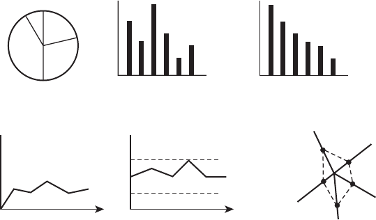
The attribute of interest is tracked as data through time, and the situation is reviewed
whenever the tracked information falls outside of the upper or lower limits. The Kiviat
chart shows the data points for multiple attributes or dimensions of interest; the example
in Figure 13.2 shows five attributes of interest and the data points representing these
areas.
In reality, we often find that the resources required to perform the monitoring is
underestimated. Running regular project meetings is a very time-consuming activity.
The analysis of gathered information may require some skilled statisticians. The very
tasks of project monitoring themselves may require the first project adjustment as we
realize the shortage of skilled data analysis resources.
Based on the monitored information, the project manager and the team would then
collectively make decisions on whether the observations indicate a need for a change.
13.2.4 Adjusting
Making adjustments is a crucial step in project management. As mentioned earlier, the
chance that a project requires no change is very small. If the monitoring process indicates
any need for adjustment, then the project management team must take timely actions.
The areas that need change may be many and varied. However, the most likely instru-
ments for adjustment that are available to the project management are the following:
n
Resources
n
Schedule
n
Project content
There is usually a trade-off decision that needs to be made among these three items,
which are tightly coupled. The resources are directly under the control of the project
management. For the most part, projects are usually in need of more resources. When
more resources are added to the projects, the timing of such additions is very impor-
Figure 13.2 Visualization and reporting of information.
Pie chart HistogramPareto diagram
Upper
limit
Lower
limit
Time
Time chart Control chart Kiviat chart
13.2 The Project Management Process
273
91998_CH13_Tsui.indd 273 1/5/13 10:01:59 AM

tant. As was well explained in Frederick Brooks’ The Mythical Man-Month (1995), add-
ing human resources to rescue schedules may often result in the reverse effect. New
employees may slow down the existing, experienced workers on the project because of
the amount of time the experienced people would have to take away from their assigned
work to explain and bring the new person on board. Similarly, introducing a new tool
or a new process at the wrong time can produce the reverse effects of elongating the
time and cost. This does not mean that project adjustments that call for more resources
should be ignored. The more the tasks are independent, the easier it is to add resources
because there are fewer coupling concerns to consider. The project management team
only needs to analyze the timing and the type of resource addition.
In contrast, there are times when resources are reduced. An example of human
resource addition and reduction that often happens in a software project would be
temporary testers who are brought on board to perform well-planned and scripted tests
but are released after the testing has been completed. This is a planned increase and
decrease of human resources. The more familiar cases are the nonplanned situations
where a schedule crunch or an unexpected change in project content forces the proj-
ect team to consider adjustments in resources. Assuming the schedule crunch means
that the schedule must be maintained but other parameters may change, then adding
resources is one possible solution and must be seriously considered. There are times
when a crucial human resource may drop off from the project. Then the project manage-
ment team must consider the possibilities of adjusting either the schedule or the project
content or both. Doing nothing and just asking the remaining people to bear the brunt
may only work once or only for a short period of time. For the most part, the project man-
agement team must consider some actions against the schedule or against the project
content when there is a resource change.
Another scenario is that a schedule needs to be kept intact or even shortened but lost
resources cannot be replaced or added quickly enough. That leaves only the option of
a reduction of project content. Reducing project content late in the project cycle, much
like adding human resources, is not trivial. A designed and coded functional area that
has some level of coupling to other parts of the software cannot easily be taken out
without careful consideration of the other interrelated areas. The time and effort spent
in reducing the project content in order to keep or shorten a schedule may in fact cre-
ate additional work and increase the schedule. In the event that more skilled resources
can be added very quickly and in time, then that may be a better solution than reducing
project content. There are times when customers flatly ask for a schedule reduction due
to increased competition, or when the upper management of a software development
organization may request an earlier product release than planned due to unplanned
external events. In such cases, a change in schedule will affect and most likely require
adjustments to resources or to product content or both. Again, schedule changes are
often unplanned and require that an appropriate adjustment is made quickly.
Often there are also changes in project content that occur after the project require-
ments are set and the project is organized to start. Inevitably, it is the customer or the
user who asks for a change or an addition. Sometimes it is just human error or the result
of seeing some prototype function and having a better understanding. We have already
discussed possible effects of late reduction of the project contents. Additions or changes
274 Chapter 13 Software Project Management
91998_CH13_Tsui.indd 274 1/5/13 10:01:59 AM

to project content are also time sensitive. In any case, most of the changes in project
content would require an adjustment in either schedule or resources or both.
These three parameters—resources, schedule, and project content—are often the
three key factors that project managers focus on during the monitoring and the adjusting
phases. Changing one usually affects the other two. Notice that another familiar attribute
in software engineering, software quality, has not been brought into the adjustment and
trade-off discussion. This is because software quality level, once agreed upon, should be
tracked but should rarely be an element offered in the adjustment and trade-offs of the
software project. Software engineers and management should be extremely careful not
to trade quality for schedule or for other parameters.
13.3 Some Project Management Techniques
There are many specific techniques involved in each of the four POMA phases. Some
require extremely deep technical knowledge and others demand great social skills. In
this section, we will focus on four commonly needed project management skills: (1)
project effort estimation, (2) work breakdown structure, (3) project status tracking with
earned value, and (4) developing measurements and metrics. The first two of them are
techniques needed in the planning and organizing phases, and the third is needed
in the monitoring phase. The fourth is needed for part of planning and for monitor-
ing. Additional details on software project management techniques can be found in
Kemerer (1997).
13.3.1 Project Effort Estimation
Estimating the software project effort has always been a difficult task, especially for the
new managers who come up from the ranks of technical positions. Many would still say
that while more rigor is needed, effort and cost estimation is an art that requires a lot of
past experience. This experience relates to knowing what to consider, how much extra
buffer needs to be put in, and how much buffer can be tolerated by the business.
In estimating software project effort, there must be some inputs that describe the
project requirements. The accuracy and the completeness of these inputs is a significant
problem. Because the inputs themselves are mostly estimates, it becomes necessary to
convert them into a single numerical number expressed in some unit of measurement
such as person-months. After the effort has been expressed in some units, the problem
of uniformity must be faced. In other words, one person-month may vary dramatically
depending on the skill level of the assigned person. In spite of these problems, it is still
necessary to estimate the project effort and put a plan together. With so much uncer-
tainty, it is not difficult to see why monitoring and adjustment phases are crucial to
project management.
In general, the estimation may be viewed as a set of project factors that may be com-
bined in some form to provide the effort estimate. The following general formula can be
used:
Units of effort = a + b(size)
c
+ ACCUM(factors)
13.3 Some Project Management Techniques
275
91998_CH13_Tsui.indd 275 1/5/13 10:01:59 AM

The units of effort are often person-months or person-days. There are several constants
and variables that are estimated. The constant, a, may be viewed as the base cost of doing
business. That is, every project has a minimum cost regardless of the size and the other
factors. This cost may include administrative and support costs such as telephone, office
space, and secretarial staff. This constant is attained after some amount of experimenta-
tion. The variable size is an estimate of the final product size in some units, such as lines of
code. The constant b is a figure that linearly scales the size variable. The constant c allows
the estimated product size to influence the effort estimation in some nonlinear form.
The constants b and c are derived through experimentation with past projects. The term
ACCUM(factors) is an accumulation of multiple factors that further influence the project
estimation. The function ACCUM may be an arithmetical sum or an arithmetical prod-
uct of a list of factors, such as technical, personnel, tools, and process factors, and other
constraints that influence the project. We will discuss two specific approaches to effort
estimation that may be viewed as some derivative of this general formula. A third effort-
estimation technique addresses only a limited portion of the general formula and will be
introduced for the object-oriented development paradigm later in this chapter.
COCOMO Estimation Models The first estimation model we will look at here is the
constructive cost model (COCOMO) approach, which originated in the work of Barry
Boehm. Boehm has modified and extended his original COCOMO to COCOMO II (Boehm
2000). Here we will provide only a summary discussion of COCOMO. The original
COCOMO includes three levels of models: a macro, an intermediate, and a micro. We will
utilize the intermediate level here as an illustration and show the overall COCOMO esti-
mation process. The following is a summary of the steps in COCOMO estimation.
1. Pick an estimate of what is considered as three possible project modes: organic
(simple), semidetached (intermediate), and embedded (difficult). The mode is
picked based on a consideration of eight project characteristics, which are dis-
cussed later. The choice of mode will determine the particular effort estimation
formula, which will also be discussed later in this section.
2. Estimate the size of the project, in thousand lines of code (KLOC). Later models in
COCOMO II allowed other metrics such as function point.
3. Review 15 factors, known as cost-drivers, and estimate the amount of impact each
factor will have on the project.
4. Determine the effort for the software project by inserting the estimated values
into the effort formula for the chosen mode.
The mode of the project is chosen based on the following eight parameters:
1. The team’s understanding of the project objectives.
2. The team’s experience with similar or related projects.
3. The project’s need to conform with established requirements.
4. The project’s need to conform with established external interfaces.
5. The need to develop the project concurrently with new systems and new opera-
tional procedures.
276 Chapter 13 Software Project Management
91998_CH13_Tsui.indd 276 1/5/13 10:01:59 AM

6. The project’s need for new and innovative technology, architecture, or other con-
straints.
7. The project’s need to meet or beat the schedule.
8. Project size.
This first step of choosing the mode is a nontrivial task because no software proj-
ect falls neatly into a single category. The three modes of organic, semidetached, and
embedded may be roughly equated to simple, intermediate, and difficult projects,
respectively. Most of the projects will have a mix of project characteristics. For example,
the eighth parameter, “project size,” may be small, but the seventh parameter, “need to
meet or beat the schedule,” may be very stringent for the specific software project. Even
just considering these two characteristics, it would be difficult deciding whether a proj-
ect is simple or intermediate. Imagine the difficulty of making a decision on the project
mode when a software project has a mixture of eight characteristics. After considering all
of them, a project mode has to be determined. Here again some past experience would
come in handy. Also, within an organization that has a history of project management
data, a new project manager may be able to consult the organization’s project database.
Once the project mode is determined, an estimation formula needs to be chosen. The
following are the corresponding estimation formulas for the three modes, with the effort
unit indicated in person-months:
Organic: Effort = [3.2 3 (size)
1.05
] 3 PROD (f ’s)
Semidetached: Effort = [3.0 3 (size)
1.12
] 3 PROD (f ’s)
Embedded: Effort = [2.0 3 (size)
1.20
] 3 PROD (f ’s)
Thus, based on the eight parameters, if we decide that the project is simple (organic),
the effort for the organic mode will be estimated with the equation Effort = 3.2 3 (size)
1.05
.
This estimation equation provides the basic estimation of project effort in person-
months, and it is the first level of estimation.
The next level of estimation in COCOMO is to consider 15 additional project factors,
called cost-drivers. PROD (f ’s) is an arithmetic product function that multiplies the 15
cost-drivers. Each of these 15 cost-drivers has a range of numerical values, ranging from
very low to extra high. These 15 cost-drivers may be categorized into four main groups:
n
Product attributes
1. Required software reliability
2. Database size
3. Product complexity
n
Computer attributes
4. Execution time constraint
5. Main memory constraint
6. Virtual machine complexity
7. Computer turnaround time
n
Personnel attributes
8. Analyst capability
13.3 Some Project Management Techniques
277
91998_CH13_Tsui.indd 277 1/5/13 10:01:59 AM

9. Applications experience
10. Programmer capability
11. Virtual machine experience
12. Programming language experience
n
Project attributes
13. Use of modern practice
14. Use of software tools
15. Required development schedule
Table 13.2 shows the values that these 15 cost-drivers may take on. The project
manager or the person given the responsibility of project estimation would review all
15 cost-drivers and the range of values for each one. Note that different cost-drivers
have different ranges of values. For example, consider cost-driver 1, required software
reliability. The lowest value is 0.75 and the highest is 1.40. If this cost-driver is deemed to
be very low or less than 1, it will lower the PROD (f ’s), and if it is deemed to be very high
or greater than 1, it will increase the PROD (f ’s). The nominal value 1.0 will not affect the
overall arithmetic product PROD (f ’s). Note that cost-driver 8, analyst capability, has 1.46
as its lowest value because low analyst capability would require more effort. The highest
value for analyst capability is 0.71 because high analyst capability would lower the effort.
Thus PROD (f ’s) may be viewed as the mechanism that allows another level of adjust-
ment to the initial project estimate provided by the earlier organic, semidetached, and
embedded effort estimation equations.
Table 13.2 COCOMO Cost-Driver Values
Cost-Drivers Very Low Low Nominal High Very High Extra High
1 0.75 0.98 1.0 1.15 1.40 —
2 — 0.94 1.0 1.08 1.16 —
3 0.70 0.85 1.0 1.15 1.30 —
4 — — 1.0 1.11 1.30 1.65
5 — — 1.0 1.06 1.21 1.66
6 — 0.87 1.0 1.15 1.30 1.56
7 — 0.87 1.0 1.07 1.15 —
8 1.46 1.19 1.0 0.86 0.71 —
9 1.29 1.13 1.0 0.91 0.82 —
10 1.42 1.17 1.0 0.86 0.70 —
11 1.21 1.10 1.0 0.90 — —
12 1.14 1.07 1.0 0.95 — —
13 1.24 1.10 1.0 0.91 0.82 —
14 1.24 1.10 1.0 0.91 0.83 —
15 1.23 1.19 1.0 1.04 1.10 —
278 Chapter 13 Software Project Management
91998_CH13_Tsui.indd 278 1/5/13 10:01:59 AM

The difficulties with COCOMO include the choosing of the particular project mode
based on the 8 parameters, the estimation of product size, and the considerations of the
15 cost-drivers. These all require some past experience. Therefore, almost all experienced
managers would attach some amount of buffers to the estimate.
While the basic principles are still the same, the early 1980s version of COCOMO has been
significantly modified and has evolved into COCOMO II. In the past 20 years, the develop-
ment process has changed from the traditional waterfall model to more iterative processes,
the development technology has moved from structured programming to object-oriented
programming, and the usage operational environment has evolved from batch to transac-
tional to highly interactive online web. The development tools have also grown from simple
compilers and linkers to a fully integrated toolkit that combines design and programming
logic, database, network middleware, and user-interface development. COCOMO II has
been modified to include these changes. We will only provide a brief update of COCOMO II
here. It has three models for estimating at different stages of the software project:
n
Creating early estimates during prototype stage
n
Making estimates after the requirements are captured, during the early design stage
n
Making estimates after the design is complete and coding has started
COCOMO II does still ask for an estimate of the size, which can now take on one of
the three metrics:
n
Thousand lines of code (KLOC)
n
Function point
n
Object point
Like lines of code, function point is an estimation of the size of the software project;
it is discussed in the next section. Object point is another estimation of the project size,
much like function point.
COCOMO II has 29 factors to consider instead of the 3 modes and 15 cost-drivers.
Much like the previous 15 cost-drivers, these 29 factors are grouped into the following
5 categories:
n
Scale factors
n
Product factors
n
Platform factors
n
Personnel factors
n
Project factors
Within each of these, there are five scale factors, five product factors, three platform
factors, six personnel factors, and ten project factors.
Research on software project estimation and, specifically, COCOMO II research and
tool development, are heavily pursued at the University of Southern California. (See the
reference to its website in the Suggested Readings section.)
Function Point Estimation The lines-of-code unit of measure has dominated the
software size-estimating arena for many of the early software engineering years. But it
has had its share of problems, and many different metrics have been proposed along the
13.3 Some Project Management Techniques
279
91998_CH13_Tsui.indd 279 1/5/13 10:01:59 AM

way. Function point was first introduced by Albrecht and Gaffney (1983) in the 1980s.
It has gained popularity and is an alternative to the lines-of-code metric for size of a
software project. While many improvements and extensions have been made to this
technique, we will describe the original version here.
Five components of software are considered in the function point estimation pro-
cess:
1. External inputs
2. External outputs
3. External inquiries
4. Internal logical files
5. External interface files
Each component is assigned a weight, based on three possible descriptions of the
project:
1. Simple
2. Average
3. Complex
Table 13.3 shows the weights that would be assigned to each of the components
based on the assumed complexity of the project. Thus if a project is assumed to be a
simple one, the number of estimated external inputs would be multiplied by the weight
3 and the estimated number of external outputs would be multiplied by the weight 4
and so on. The unadjusted function point (UFP) for a simple project would be the arith-
metic sum of these weighted components as follows.
UFP = (number of inputs 3 3) + (number of outputs 3 4) + (number of inquiries
3 3) + (number of logical files 3 7) + (number of interface files 3 5)
The unadjusted function point estimate hinges on how accurately the numbers of
each of the five components are estimated and the project complexity assumption. Here
again, some past software project experience would be very helpful.
Once again, as in COCOMO, there are a number of factors influencing decision. There
are 14 technical complexity factors that need to be considered, with each taking on a
value of 0 through 5:
1. Data communications
2. Distributed data
Table 13.3 Function Point Weights
Software Components Simple Average Complex
External inputs 3 4 6
External outputs 4 5 7
External inquiries 3 4 6
Internal logical files 7 10 15
External interface files 5 7 10
280 Chapter 13 Software Project Management
91998_CH13_Tsui.indd 280 1/5/13 10:01:59 AM

3. Performance criteria
4. Heavy hardware usage
5. High transaction rates
6. Online data entry
7. Online updating
8. Complex computations
9. Ease of installation
10. Ease of operation
11. Portability
12. Maintainability
13. End-user efficiency
14. Reusability
The sum of these 14 technical complexity factors has a value ranging from 0 (0 3 14
= 0), to 70 (5 3 14 = 70). If the technical complexity factor is judged to be nonessential,
then it would be given a value of 0; if it is thought to be extremely relevant, it is given a
value of 5. A total complexity factor (TCF) is then calculated based on the sum of these
14 technical complexity factors:
TCF = 0.65 + [(0.01) 3 (sum of 14 technical complexity factors)]
Thus TCF may have a value ranging from 0.65 to 1.35. Finally, the function point (FP)
is defined as the arithmetic product of unadjusted function point (UFP) and total com-
plexity factor:
FP = UFP 3 TCF
Note that because TCF may vary between 0.65 and 1.35, TCF provides the adjustment
factor for the initial estimation, which is the UFP. Again, if we believe that there needs to
be more buffering than what TCF’s 1.35 allows, then extra buffering may be added.
Function point is only an estimation of the size. To convert the function points into
an effort estimate, we need to have some idea of the productivity of the group. That is,
we still need to convert function points into some form of person-month. Assuming that
there is an organizational database that allows us to state that the productivity figure may
be estimated at 25 function points per person-month, we can calculate the effort estima-
tion, in person-months, for a project estimated at ZZZ function points as follows:
Effort = (ZZZ function points) / (25 function points/person-month)
As in other estimation techniques, it is very difficult to have consistency across dif-
ferent organizations and estimators with function points. A total of 100 function points
should mean the same regardless of who stated it. In order to achieve such consistency
within the software engineering field, there is an organization called International
Function Point Users Group (IFPUG), which provides both education and information
exchanges on function points. Since the inception of this estimation technique, the
field of software engineering has evolved considerably. Similar to COCOMO II, there are
many FP extensions proposed and tried by various groups.
13.3 Some Project Management Techniques
281
91998_CH13_Tsui.indd 281 1/5/13 10:01:59 AM

A Simple OO Effort Estimation Lorenz and Kidd (1994) introduced a very simple tech-
nique for those who want to estimate with object-oriented (OO) objects. This technique
has some resemblance to the function point approach in that it is based on an estimated
number of components or classes that would be in the final software product and associ-
ating some weight to the classes. The number of estimated OO classes may be viewed as
the size parameter in the general formula introduced earlier. The process for this estima-
tion technique is summarized in the following four steps:
1. Estimate the number of classes in the problem domain. This may be done by
studying and analyzing the requirements.
2. Categorize the types of user interfaces and assign weights as follows:
No user interface (UI) 2.0
Simple, text-based UI 2.25
Graphical UI (GUI) 2.5
Complex GUI 3.0
These weights are derived from past experiences with many OO projects and from
examining the effects the type of UI had on numbers and types of classes.
3. Multiply the estimated number of classes in Step 1 by the weight associated with
the type of user interface that is projected for this project. Add this arithmetic
product to the original estimate of classes to get a new estimate of total classes
that may be in the final product.
4. Multiply the estimated total number of classes from Step 3 by a number between
15 and 20, a productivity estimate of the number of person-days required to
develop a class.
In order to carry out these four steps, there are several assumptions that must be
made—for example, the estimated number of classes in Step 1 or the number of person-
days needed to develop a class. Such decisions would require not only prior project
experience but a certain amount of design in mind. The project manager thus needs
to sit down with the designers and agree on the estimated number of classes and the
projected user-interface category.
For example, let’s assume that the initial estimate is 50 classes and the user interface is
considered to be complex GUI. We then would multiply 50 by a factor of 3.0, which gives
us 150 additional classes. Adding the 150 to 50, we have a new estimate of total final
classes of 200. Assuming the productivity is 18 person-days per class, the effort estimate
would then be 200 3 18 = 3600 person-days. The person-day unit for effort may be con-
verted to a person-month unit, if desired.
The important thing to remember is that all of these effort estimates are indeed just
estimates. Project managers must apply some intelligence and appropriate amount of
buffer to these calculations before conveying any effort estimates to the customers or
the users or even to their own management.
282 Chapter 13 Software Project Management
91998_CH13_Tsui.indd 282 1/5/13 10:01:59 AM

13.3.2 Work Breakdown Structure
Estimating a complete project work effort is an important but difficult task. It can be
made a little easier if the overall project is divided into smaller portions that provide a
basis for the rest of planning activities such as scheduling and staff assignments. The
work breakdown structure (WBS) is a depiction of the project in terms of discrete subac-
tivities that must be conducted to complete the project. WBS first looks at the required
deliverables of the software project. Then, for each of the artifact that needs to be deliv-
ered, a set of high-level tasks that must be performed to develop the deliverable is identi-
fied. These tasks are also presented in an ordered fashion so that task scheduling can be
accomplished from the WBS. The following is a framework for performing WBS:
1. Examine and determine the required external deliverables of the software project.
2. Identify the steps and tasks required to produce each of the external deliverables,
including the tasks that would be required to develop any intermediate internal
deliverable needed for the final external deliverable.
3. Sequence the tasks, including the specification of tasks that may be performed in
parallel.
4. Provide an estimate of the effort required to perform each of the tasks.
5. Provide an estimate of the productivity of the personnel that is most likely to be
assigned to each task.
6. Calculate the time required to accomplish each of the tasks by dividing the effort
estimate by the productivity estimate for each task.
7. For each external deliverable, lay out the timeline of all the tasks needed to pro-
duce that deliverable and label the resources that will be assigned to the tasks.
For example, let’s consider an external deliverable of test scenarios for a small soft-
ware project that is estimated to be around 1000 lines of code or involve approximately
100 function points. As part of the WBS, we need to first list the tasks that are required to
produce this deliverable. Such a list may look as follows:
n
Task 1: Read and understand the requirements document.
n
Task 2: Develop a list of major test scenarios.
n
Task 3: Write the script for each of the major scenarios.
n
Task 4: Review the test scenarios.
n
Task 5: Modify and change the scenarios.
These five tasks appear to be sequential, and they are at a macro level. However, we
can probably gain some speed if some of the major tasks can be subdivided into smaller
pieces and be performed in parallel. It would also seem that as some of the test scenarios
are developed they can be reviewed and fixed. So, we may consider some overlapping of
subtasks when we are ready to convert the WBS to a schedule. For illustration purposes,
we divide Task 3 into Task 3a, Task 3b, and Task 3c to represent three equally divided sub-
tasks of the script-writing activities. Task 4 can be decomposed to Task 4a, Task 4b, Task
4c to match the three Task 3 subactivities. Similarly, Task 5 can be subdivided into Task
13.3 Some Project Management Techniques
283
91998_CH13_Tsui.indd 283 1/5/13 10:01:59 AM
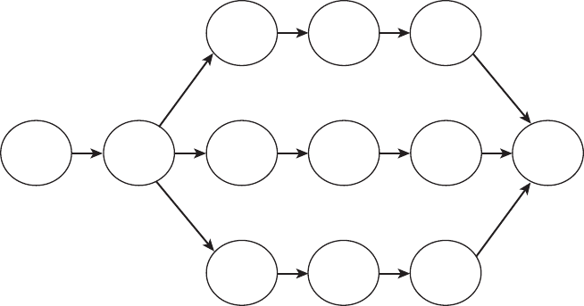
5a, Task 5b, and Task 5c to match the three subactivities of Task 4. Figure 13.3 shows
what the WBS network of tasks for this deliverable would look like. Clearly illustrating the
WBS and the sequence along with which tasks may be carried out in parallel, this figure
can become a very convenient tool when the number of tasks and sequences is large.
The next step is to estimate the effort required to complete each of the tasks. For
Task 1, we need to estimate the effort required to read and understand the requirements
of a project that is about 1000 lines of code or about 100 function points. For Task 2, we
need to estimate the number of test scenarios that would need to be developed and
how long it would take to come up with such a list. For Tasks 3a, 3b, and 3c, we need
to estimate the effort needed to develop the test scripts for one-third of the scenarios.
Similarly, we need to estimate the effort required to review one-third of the scenario
scripts for Tasks 4a, 4b, and 4c. Estimating effort needed for Tasks 5a, 5b, and 5c would be
very difficult because they depend on how many modifications are required as a result of
Tasks 4a, 4b, and 4c. Nevertheless, all these initial estimates must be done. Fortunately,
we do get to adjust our project because, as discussed in Section 13.2.4, adjustment is an
intricate part of the four phases of project management. After these initial estimations
have been made, we need to make an assumption and estimate the level of competency
or the productivity of the people who will be assigned to all of these tasks. Then the
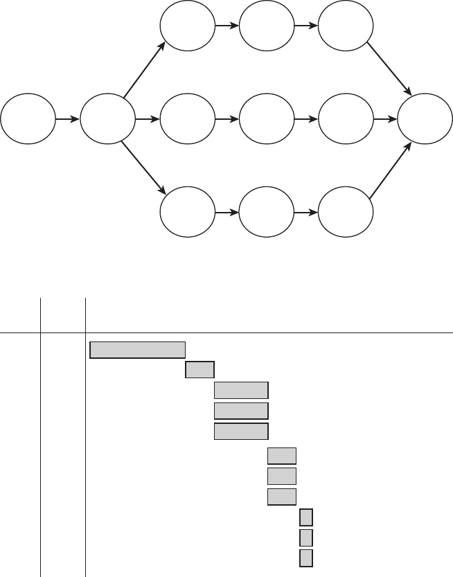
estimated time for each of the tasks in Figure 13.3 can be computed by dividing the
estimated effort by the estimated productivity. Figure 13.4 shows the same WBS tasks
with the estimated time units required to perform these tasks and the order of the tasks.
From this information, we can establish the preliminary schedule as shown in Figure
13.5. Note that there are three main parts to the schedule: (1) the tasks, (2) the human
resource assignment, and (3) the time units.
The transformation from WBS task network to an initial schedule directly moved two
items: the tasks and the time units. The middle column in Figure 13.5 lists the presumed
staff resource assignment, an important consideration that is the source for the produc-
Figure 13.3 A WBS network of tasks.
Task 3a Task 4a Task 5a
Task 3bTask 2Task 1 Task 4b Task 5b End
Task 3c Task 4c Task 5c
284 Chapter 13 Software Project Management
91998_CH13_Tsui.indd 284 1/5/13 10:02:00 AM
tivity assumptions used to compute and estimate the time units required to complete
the task. Earlier, it was also mentioned that the tasks may overlap. Once the initial sched-
ule is formulated, the project management may look for the possibilities of overlapping
the tasks, besides the already shown parallel tasks. In this example, the end of Task 1 and
the beginning of Task 2 may overlap. The overlapping of subtasks, Task 3a, 3b, and 3c
with Task 4a, 4b, and 4c would be a lot trickier because a different person—a person who
is committed to writing test scripts but may not have completed the writing task—must
Figure 13.4 Task network with estimated time units.
Task 3a
6
Task 4a
2
Task 5a
1
Task 3b
6
Task 2
2
Task 1
12
Task 4b
2
Task 5b
1
End
Task 3c
6
Task 4c
2
Task 5c
1
Figure 13.5 Initial schedule estimate.
Tasks Person
Time
1
2
3a
3b
3c
4a
4b
4c
5a
5b
5c
X, Y, Z
X, Y, Z
X
Y
Z
Z
X
Y
X
Y
Z
12 units
2
6
6
6
2
2
2
1
1
1
13.3 Some Project Management Techniques
285
91998_CH13_Tsui.indd 285 1/5/13 10:02:00 AM

perform the review. Without including the column on resource assignment in the initial
schedule, these kinds of subtleties may escape the project planners. In our example here,
we have chosen to keep everything simple and showed no overlap of tasks in the initial
schedule.
Considering all the different types of estimations that went into the task network of
Figure 13.4, we should anticipate that the first schedule shown in Figure 13.5 will need
to be modified as the project proceeds. This initial schedule should be reviewed by as
many of the project constituents as possible before the schedule may be regarded as a
planned schedule.
Work breakdown structure is an important and necessary input to the creation of the
initial schedule. Unfortunately, many software project schedules are constructed without
developing a thorough WBS, and the result is an unattainable and unrealistic project
schedule.
13.3.3 Project Status Tracking with Earned Value
Keeping track of or monitoring project status is the activity that compares what was
planned against what actually took place. There are multiple attributes of the project that
need to be tracked. Most of these are identified in the set of goals stated in the project plan.
We are constantly and periodically comparing the actual status of the attributes expressed
as project goals against what was planned. In this section we will discuss the tracking of
project efforts using the concept of earned value (EV), which was first developed by orga-
nizations inside the U.S. government. Fleming and Koppelman (2000) provide an extensive
discussion on EV.
When using the earned value management technique, the fundamental concept is to
compare the status of how much effort has been expended against how much effort was
planned to have been expended at some point in time. First we will need to understand
some basic terminology, and then an example will be provided to clarify these defini-
tions.
n
Budgeted cost of work (BCW): The estimated effort for each of the work tasks.
n
Budgeted cost of work scheduled (BCWS): The sum of the estimated effort of all the
tasks that were scheduled to be completed at a specific status-checking date. (This is
the sum of all the BCWs that were scheduled, according to the plan, to be completed
at a specific status-checking date.)
n
Budget at completion (BAC): The estimate of the total project effort; it is the sum of all
the BCWs.
n
Budgeted cost of work performed (BCWP): The sum of the estimated efforts of all the
tasks that have been completed at the specific status-checking date.
n
Actual cost of work performed (ACWP): The sum of the actual efforts of all the tasks
that have been completed at a specific status-checking date.
A factor that should be remembered is that BCWS, BCWP, and ACWP are all stated in
terms of a specific status-monitoring date. Thus those values will change relative to the
status date.
Table 13.4 shows an example of estimated efforts and actual efforts expended as
of a specific date, which is 4/5/2012. The date format used here is month/day/year. The
286 Chapter 13 Software Project Management
91998_CH13_Tsui.indd 286 1/5/13 10:02:00 AM

efforts are measured in person-days (Pers-days). Each task has a budgeted cost of work,
and the BCWs for the six tasks are shown in the column showing estimated effort. For
example, for Task 4 the BCW is 25 Pers-days. The sum of this column, or the sum of the
BCWs, is the budget at completion:
BAC = 10 + 15 + 30 + 25 + 15 + 20 = 115 Pers-days.
Now let us look at the three values that are computed relative to the status taking
date, which in this case is 4/5/2012. By examining the column showing the estimated
completion date, the BCWS as of 4/5/2012 includes Tasks 1 and 2. The BCW for Tasks 1
and 2 respectively are 10 and 15 Pers-days:
BCWS = 10 + 15 = 25 Pers-days
We next look at how much of the estimated work is completed on 4/5/2012. This can
be found by examining the actual completion date column. We see that tasks 1, 2, and 4
have been completed. These three completed tasks had been estimated to take 10, 15,
and 25 Pers-days:
BCWP = 10 + 15 + 25 = 50 Pers-days
The actual effort expended for those tasks that were completed on 4/5/2012 is found
by looking at the actual completion date and taking the effort values for those com-
pleted tasks from the column entitled “Actual Effort Spent So Far in Pers-days.” The actual
effort for completed Tasks 1, 2, and 4 are 10, 25, and 20 Pers-days respectively:
ACWP = 10 + 25 +20 = 55 Pers-days.
The next step is to define earned value in terms of the earlier definitions. Earned value
is an indicator that will tell us how much of the estimated work is completed on a specific
date. It compares the sum of all the estimated efforts of the completed tasks as of the
status date against the sum of the estimated efforts of all the tasks:
EV = BCWP / BAC
In terms of our example, EV = 50 / 115 = 0.43. We may interpret this to mean that the
project is 43% complete as of 4/5/2012.
There are two more status indicators that can be derived from the definitions. These
are variance indicators that, once again, compare the planned or estimated value against
Table 13.4 Earned Value Example Date: 4/5/2012
Work Tasks
Estimated Effort in
Pers-days
Actual Effort Spent
So Far in Pers-days
Estimated
Completion Date
Actual
Completion Date
1 10 10 2/5/2012 2/5/2012
2 15 25 3/15/2012 3/25/2012
3 30 15 4/25/2012
4 25 20 5/5/2012 4/1/2012
5 15 5 5/25/2012
6 20 15 6/10/2012
13.3 Some Project Management Techniques
287
91998_CH13_Tsui.indd 287 1/5/13 10:02:00 AM

the actual value. The first one is a schedule variance (SV) indicator, which is defined as
the difference between estimated efforts of the tasks that have been completed by the
status date and the estimated efforts of the tasks that were scheduled or planned to have
been completed by the status date:
SV = BCWP 2 BCWS
In our example, on 4/5/2012, BCWP is 50 Pers-days, and BCWS is 25 Pers-days. Thus
SV = 50 2 25, or 25 Pers-days. We may interpret the project status as 25 Pers-days ahead
of schedule from an effort perspective.
The second variance indicator is the cost variance (CV), which is defined as the differ-
ence between the estimated efforts of the tasks that have been completed at the status
date and the actual efforts expended for the tasks that have been completed at that
status date.
CV = BCWP 2 ACWP
In our example, on 4/5/2012, BCWP is 50 Pers-days, and ACWP is 55 Pers-days. Thus
CV = 50 255, or 25 Pers-days. In this case, on 4/5/2012, we have 5 Pers-days of effort
cost overrun.
The earned value management system provides us with a concrete way to monitor
project status from a cost/effort perspective. However, the schedule variance is not an
indicator of calendar time schedule but an effort schedule. Clearly more indicators may
be constructed from this basic set of definitions, but we will not include them here. We
have found that the set EV, SV, and CV provide a good indicator of project status, but we
must still remember to look beyond the numbers, ask questions, and delve into other
parameters when monitoring a software project. As a final reminder, if the monitored
information indicates potential project problems, then adjustments must be made. Do
not wait for some project-saving event to occur on its own. Project managers rarely have
such luck.
13.3.4 Measuring Project Properties and GQM
We have discussed the need to set goals for a software project during the planning stage
so that these goals can be tracked and checked to see if they have been met. The goals
are stated in terms of such properties as schedule, cost, productivity, maintainability,
defect quality, and so on. Clearly, the specific characteristics of interest must be well
defined before any measurement of can take place. Besides setting and tracking goals,
the reasons for measurement include the following:
n
Characterization: Allows us to gather information about and intelligently describe a
property.
n
Tracking: Allows us to gather information about a property through such parameters
as time or process steps.
n
Evaluation: Allows us to analyze the property via gathered information.
n
Prediction: Allows us to correlate properties and to extrapolate or conjecture about the
property based on the gathered information.
n
Improvement: Allows us to identify areas of improvement based on an analysis of gath-
ered information.
288 Chapter 13 Software Project Management
91998_CH13_Tsui.indd 288 1/5/13 10:02:00 AM

It is critical for software engineers to join the rest of the engineering communities
to adopt measurement and quantitative analysis. Measurement is a vital part of quan-
titative management. Software (product or project) measurement is a mapping of an
attribute of a software product or project to some set of numeric or symbolic entities. It
can be deceivingly tricky to come up with good measurements. The following is a short
guideline to assist you:
1. Conceptualize the entity of interest such as the software product or project, the
members of the project team, etc.
2. Clearly define the specific attributes of interest such as product design quality,
programmer productivity, and project cost, etc.
3. Define the metrics to be used for each attribute of interest such as defects per class
in a UML class design diagram, lines of code developed per programmer month,
dollars expended per project month, etc.
4. Devise the mechanism to capture the metrics; this could include manually count-
ing the number of defects in each designed class in the UML diagram.
Basili and Weiss (1984) introduced the Goal-Question-Metric (GQM) approach to
software metrics. GQM has been used quite successfully by many organizations. This
approach defines a measurement model based on three levels:
n
Conceptual level: Establish a goal. For instance, “Improve the time to locate a software
code problem.”
n
Operational level: Develop a list of questions related to the goal. For example, “How
does the program complexity influence software debugging time?”
n
Quantitative level: Develop metrics. These could include the number of control loops
in the program for control complexity and the number of person-minutes spent on
debugging efforts.
Next, we will briefly touch on the theory of metrics to further guide us in the estab-
lishment of valuable metrics. The extensive detail regarding the mathematic mapping
theory of metrics is too large in scope to cover in this text. We will, however, discuss the
four scale levels of metrics: nominal, ordinal, interval, and ratio.
The nominal level allows us to distinctively categorize a property. For example, con-
sider the case of measuring the number of software defects by source categories such as
design, code, test, integration, and packaging. The danger with this set of categories as a
metric is that a defect may originate from both design and coding. We must ensure that
every defect is assigned only to a unique category for the metric to be nominal.
The ordinal level provides an ordering of the property. For example, when one is mea-
suring customer satisfaction with categories of very satisfied, satisfied, neutral, not satis-
fied, and very dissatisfied. This metric is more than just nominal because it also provides
an ordering of very satisfied to very dissatisfied.
The third level of metrics is the interval level. The interval level allows us to describe
equal intervals. For instance, program A has 200 function points, which is 20 function
points more than program B. This difference is the same as program C with 70 function
points, while program D has 50 function points. The difference, 20 function points, is
considered to have equal intervals. Note that we could not have performed this type of
13.3 Some Project Management Techniques
289
91998_CH13_Tsui.indd 289 1/5/13 10:02:00 AM

operation with ordinal-level metrics. Consider the difference between very satisfied and
satisfied and the difference between satisfied and neutral in the ordinal metric example.
These two differences are not necessarily of equal intervals.
The final metric, ratio, allows us to compare the ratio of two measurements because
it has a defined 0 in the metric. For example, it makes sense to say program A, which has
100 lines of source code, is 4 times the size of program B, which has 25 lines of source
code. This is a result of the established 0 line of code as minimum size. The ratio scale is
the highest metric level.
13.4 Summary
We first introduced the four POMA phases of software project management: (1) plan-
ning, (2) organizing, (3) monitoring, and (4) adjusting. POMA is shown to be sequential
at the macro level. However, the phases may overlap and may actually iterate among
themselves, especially between the monitoring and adjustment phases. The complex
and time-consuming planning phase is the key to project success. The monitoring phase
is also important, and all projects must be monitored until the end. When necessary, the
project manager must take actions and make the appropriate adjustments.
A general formula for effort estimation that involves several parameters is first shown.
Then the following three specific techniques related to this general formula for effort
estimation are discussed:
n
Constructive cost model (COCOMO) approach
n
Function point estimation
n
Simple OO effort estimation
The principles behind the original COCOMO estimating methodology are explained
and then its extensions and modifications into COCOMO II are introduced. The function
point estimation technique for project size is shown as an alternative to the line-of-code
estimation technique. How function point size effort may be converted to effort estima-
tion is also discussed. The OO effort estimation technique is involved with estimating the
number of key classes and the assumed productivity level of the software engineers.
Another important planning technique, work breakdown structure, is demonstrated
with a network of tasks and their respective estimated efforts. The significance of WBS
to developing an initial project schedule, in a bar chart form, is explained with an
example.
Project monitoring involves the ongoing comparison between what is planned and
what is actual. Based on this observation, project managers would have to decide on
whether any action, or adjustment, needs to be taken. Earned value management is
introduced as a viable technique for monitoring the project effort and project schedule.
This process essentially compares the planned or estimated project task efforts against
those project task efforts that were actually expended. We have explained the need for
setting goals and tracking the goals as part of project management. In order to accom-
plish those tasks, measurement is needed. GQM is introduced as a methodology, and
the scales of metrics are also discussed.
290 Chapter 13 Software Project Management
91998_CH13_Tsui.indd 290 1/5/13 10:02:00 AM

13.5 Review Questions
1. List and discuss the elements of a project plan.
2. What are the fours phases of project management?
3. What are the three components of risk management?
4. What is a Kiviat chart, and when would you use it?
5. What are the three attributes of a software project that are most often considered
for trade-off decisions for project adjustment?
6. Consider the COCOMO project effort estimation methodology.
a. What are the three project modes?
b. What are the eight project characteristics that you need to consider in
order to decide the project mode?
c. How do the 15 cost-drivers influence the initial effort estimate?
d. Consider a software project that you have estimated at 2 KLOC in size. You
believe that it should be in organic mode and that the arithmetic product
of the 15 cost-drivers or PROD (f ’s) is 1.2. What is the estimated effort in
person-months?
7. Using function point methodology, compute the unadjusted function point for an
average project that has 10 external inputs, 7 external outputs, 5 external inqui-
ries, 3 internal logical files, and 4 external interface files.
8. Assume that the total complexity factor for the software project in the previous
question is 1.1 and the productivity figure is 20 function points per person-month.
What is the function point for the project? What is the estimated effort in person-
months for the project?
9. What is WBS, and what is it used for?
10. What are the three key project status indicators, EV, SV, and CV, in earned value
project status tracking methodology?
11. What are the four scale levels of metric?
12. What is GQM?
13.6 Exercises
1. Compare and contrast a software development process with the software project
management (POMA) process.
2. Describe one activity that belongs to the organizing phase.
13.6 Exercises
291
91998_CH13_Tsui.indd 291 1/5/13 10:02:00 AM
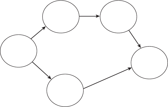
3. Consider a software project that asks you to track the grades of the entire fresh-
man class at your college, by major, by gender, and by geographical region. Pull
together a plan for this software project, including the work needed to clarify the
requirements and deliverables.
4. When would you utilize the control chart for monitoring and why? Give an exam-
ple.
5. Discuss the perils of increasing resources as a part of project adjustment.
6. Compare the list of factors considered in the effort estimation techniques of
COCOMO and of function point.
7. When we perform the arithmetic multiplication of TCF to UFP, what is the range
of adjustment (in a percentage) made to the unadjusted function point (UFP)?
8. Consider the task network illustrated in Figure 13.6, with the estimated effort
shown in units of person-months. Make the appropriate assumptions to convert
it into a project schedule.
Task B
3
Task C
7
Task A
6
Task D
5
END
Figure 13.6 A task network.
a. Explain what assumptions you need to make.
b. Use these assumptions and convert the task chart to a schedule bar chart.
9. We saw in the earned value example shown in Table 13.4 that there is more actual
effort spent than what the BCWP indicates on 4/5/2012 because that calculation
only includes the completed tasks. Suppose we invent another term called all
actual efforts spent (AAES) to include all the efforts spent as of the status date and
then use it to compute a new formula: EV9 = AAES / BAC.
a. Discuss your opinion of utilizing EV9 instead of EV.
292 Chapter 13 Software Project Management
91998_CH13_Tsui.indd 292 1/5/13 10:02:00 AM

b. Because AAES is just a redefined and expanded BCWP, do you believe the SV and
CV figures will be more representative of the true project status if we use AAES in
computing SV and CV? Why?
10. In the effort estimation of OO projects, we arithmetically multiply the counts of
estimated classes by an estimated 15 to 20 person-days per class.
a. Do you believe this is a wide enough range for the development of a class?
What would be some of the parameters you would consider about the class or
the developer before assigning a productivity figure?
b. If you were to come up with a productivity number to develop a class, what
activities (design, code, test, etc.) would you include in that estimated figure?
13.7 Suggested Readings
A. J. Albrecht and J. Gaffney, “Software Function, Source Lines of Code, and Development
Effort Prediction: A Software Science Validation,” IEEE Transactions on Software Engineer-
ing (November 1983): 639–648.
V. R. Basili and D. Weiss, “A Methodology for Collecting Valid Software Engineering Data,”
IEEE Transactions on Software Engineering 10, no. 6 (November, 1984): 728–738.
B. W. Boehm, Software Engineering Economics (Englewood Cliffs, NJ: Prentice Hall, 1981).
——, “Software Risk Management: Principles and Practices,” IEEE Software (January 1991):
32–41.
—— et al., Software Cost Estimation with COCOMO II (Upper Saddle River, NJ: Prentice Hall,
2000).
F. P. Brooks Jr., The Mythical Man-Month: Essays on Software Engineering, anniversary edi-
tion (Reading, MA: Addison-Wesley, 1995).
P. F. Drucker and N. Stone, eds., Peter Drucker on the Profession of Management (Cam-
bridge, MA: Harvard Business School Press, 1998).
Q. W. Fleming and J. M. Koppelman, Earned Value: Project Management, 2nd ed. (Newton
Square, PA: Project Management Institute, 2000).
A. J. Hayter, Probability and Statistics for Engineers and Scientists, 2nd ed. (Pacific Grove, CA:
Duxbury Press, 2002).
International Function Point Users Group (IFPUG), http://www.ifpug.org
S. H. Kan, Metrics and Models in Software Quality Engineering, 2nd ed. (Reading, MA: Addi-
son-Wesley, 2003).
C. F. Kemerer, Software Project Management: Readings and Cases (Boston, MA: Irwin
McGraw-Hill, 1997).
M. Lorenz and J. Kidd, Object-Oriented Software Metric (Upper Saddle River, NJ: Prentice
Hall, 1994).
S. McConnell, Software Project Survival Guide (Redmond, WA: Microsoft Press, 1998).
293
13.7 Suggested Readings
91998_CH13_Tsui.indd 293 1/5/13 10:02:00 AM

A. D. Meyer, C. H. Loch, and M. T. Pich, “Managing Project Uncertainty: From Variation
to Chaos,” MIT Sloan Management Review (Winter 2002): 60–67.
I. Myrtveit, E. Stensrud, and M. Shepperd, “Reliability and Validity in Comparative Studies
of Software Prediction Models,” IEEE Transactions on Software Engineering 31, no. 5 (May
2005): 380–391.
R. R. Patrashkova-Volzdoska, S. McComb, S. Green, and W. Compton, “Examining a Cur-
vilinear Relationship Between Communication Frequency and Team Performance in
Cross-Functional Project Teams,” IEEE Transactions on Engineering Management 50, no. 3
(August 2003): 262–269.
M. Rene, “Risk Management for Testers,” Software Quality Professional (June 2005): 24–
33.
J. Ropponen and K. Lyytinen, “Components of Software Development Risk: How to Ad-
dress Them? A Project Manager Survey,” IEEE Transactions on Software Engineering (Feb-
ruary 2000): 98–111.
M. Shepperd and D. Ince, Derivation and Validation of Software Metrics (Oxford, England:
Clarendon Press, 1993).
Standish Group, The Chaos Report (1994), http://net.educause.edu/ir/library/pdf
/ncp08083b.pdf, accessed 2012.
F. Tsui, Managing Software Projects (Sudbury, MA: Jones and Bartlett Publishers, 2004).
University of Southern California, Center for Software Engineering, http://sunset.usc.edu
/csse/research/COCOMOII/cocomo_main.html
H. Weihrich, “Management: Science, Theory, and Practice.” In Software Engineering Project
Management, 2nd ed., edited by R. H. Thayer (Los Alamitos, CA: IEEE Computer Society,
1997): 4–13.
C. Zucchermaglio and A. Talamo, “The Development of a Virtual Community of Practices
Using Electronic Mail and Communicative Genres,” Journal of Business and Technical Com-
munication 17, no. 13 (July 2002): 259–284.
294 Chapter 13 Software Project Management
91998_CH13_Tsui.indd 294 1/5/13 10:02:00 AM
..................Content has been hidden....................
You can't read the all page of ebook, please click here login for view all page.