
Chapter 9
Causality and Matching
9.1 Introduction
Causality is a concept that statisticians and statistical science traditionally shy away from. Recently, however, many successful attempts have been made to include the concept of causality in the statistical theory and vocabulary. A good review of the topic, from a modern event history analysis point of view, is given in Aalen et al. (2008), Chapter 9. Some of their interesting ideas are presented here.
The traditional standpoint among statisticians was that “we deal with association and correlation, not causality”; see Pearl (2000) for a discussion. An exception was the clinical trial, and other situations, where randomization could be used as a tool. However, during the last couple of decades, there has been an increasing interest in the possibility of making causal statements even without randomization, that is, in observational studies (Rubin 1974, Robins 1986).
Matching is a statistical technique, that has an old history without an explicit connection to causality. However, as we will see, matching is a very important tool in the modern treatment of causality.
Unfortunately, the models for event history analysis presented here are not implemented in R or, to my knowledge, in any other publicly available software. One exception is matched data analysis, which, except the matching itself, can be performed with ordinary stratified Cox regression.
9.2 Philosophical Aspects of Causality
The concept of causality has a long history in philosophy; see for instance (Aalen et al. 2008) for a concise review. A fundamental question, with a possibly unexpected answer, is “Does everything that happens have a cause?” According to (Zeilinger 2005), the answer is “no.”
The discovery that individual events are irreducibly random is probably one of the most significant findings of the twentieth century. Before this, one could find comfort in the assumption that random events only seem random because of our ignorance....
But for the individual event in quantum physics, not only do we not know the cause, there is no cause.
Of course, this statement must not necessarily be taken literally, but it indicates that nothing is to be taken as granted.
9.3 Causal Inference
According to (Aalen et al. 2008), there are three major schools in statistical causality: (i) graphical models, (ii) predictive causality, and (iii) counterfactual causality. They also introduce a new concept, dynamic path analysis, which can be seen as a merging of (i) and (ii), with the addition that time enters explicitly the models.
9.3.1 Graphical Models
Graphical models have a long history, emanating from (Wright 1921), who introduced path analysis. The idea was to show by writing diagrams how variables influence one another. Graphical models have had a revival during the last decades with very active research; see (Pearl 2000) and (Lauritzen 1996). A major drawback for event history analysis purposes is, according to (Aalen et al. 2008), that time is not explicitly taken into account. The idea is that causality evolves in time; That is, a cause must precede an effect.
9.3.2 Predictive causality
The concept of predictive causality is based on stochastic processes, and that a cause must precede an effect in time. This may seem obvious, but very often you see it not clearly stated. This leads sometimes to confusion, for instance, to questions like “What is the cause, and what is the effect?”
One early example is Granger causality (Granger 1969) in time series analysis. Another early example with more relevance to event history analysis is the concept of local dependence. It was introduced by Tore Schweder (Schweder 1970).
Local dependency is illustrated in Figure 9.1. A and B are events, and the superscript (c) indicates their complements, that is, they have not (yet) occurred if superscripted. This model is used in the matched data example later in this chapter. There A stands for mother dead and B means infant dead. The mother and her newborn (alive) infant are followed from the birth to the death of the infant (but at most a one-year follow-up). During this follow-up, both mother and infant are observed and the eventual death of the mother is reported. The question is whether the mother’s death influences the survival chances of the infant (it does!).
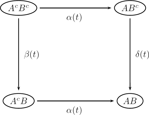
In Figure 9.1: If β(t) ≠ δ(t), then B is locally dependent on A, but A is locally independent on B: The vertical transition intensities are different, which means that the intensity of B happening is influenced by A happening or not. On the other hand, the horizontal transitions are equal, meaning that the intensity of A happening is not influenced by B happening or not. In our example, this means that mother’s death influences the survival chances of the infant, but mother’s survival chances are unaffected by the eventual death of her infant (maybe not probable in the real world).
9.3.3 Counterfactuals
In situations where interest lies in estimating a treatment effect, the idea of counterfactual outcomes is an essential ingredient in the causal inference theory advocated by Rubin (Rubin 1974) and Robins (Robins 1986). An extensive introduction to the field is given by Hernán & Robins (2012).
Suppose we have a sample of individuals, some treated and some not treated, and we wish to estimate a marginal treatment effect in the sample at hand. If the sample is the result of randomization, that is, individuals are randomly allocated to treatment or not treatment (placebo), then there are in principle no problems. If, on the other hand, the sample is self-allocated to treatment or placebo (an observational study), then the risk of confounders destroying the analysis is overwhelming. A confounder is a variable that is correlated both with treatment and effect, eventually causing biased effect estimates.
The theory of counterfactuals tries to solve this dilemma by allowing each individual to be its own control. More precisely, for each individual, two hypothetical outcomes are defined; the outcome if treated and the outcome if not treated. Let us call them Y1 and Y0, respectively. They are counterfactual (counter to fact), because none of them can be observed. However, since an individual cannot be both treated and untreated, in the real data, each individual has exactly one observed outcome Y. If the individual was treated, then Y = Y0, otherwise Y = Y1. The individual treatment effect is Y1 − Y0, but this quantity is not possible to observe, so how do we proceed?
The Rubin school fixes balance in the data by matching, while the Robins school advocates inverse probability weighting. It is possible to apply both these methods to event history research problems (Hernán, Brumback & Robins 2002, Hernán, Cole, Margolick, Cohen & Robins 2005), but unfortunately there is no publicly available software for performing these kinds of analyses, partly with the exception of matching, of which an example is given later in this chapter. However, with the programming power of R, it is fairly straightforward to write our own functions for specific problems. This is, however, out of the scope of this presentation.
The whole theory based on counterfactuals relies on the assumption that there are no unmeasured confounders. Unfortunately, this assumption is completely untestable, and even worse, it never holds in practice. Does this mean that the whole theory of causal inference is worthless? No, it does not, because the derived procedures are often sound even without the attribute “causal.” But claiming causality is an exaggeration in most circumstances. What we can hope for is the elimination of the effects of the measured confounders.
9.4 Aalen’s Additive Hazards Model
In certain applications it may be reasonable to assume that risk factors acts additively rather than multiplicatively on hazards. Aalen’s additive hazards model (Aalen 1989, Aalen 1993) takes care of that.
For comparison, recall that the proportional hazards model may be written
where r(β, xi) is a relative risk function. In Cox regression, we have: r(β, xi) = exp(βTxi),
The additive hazards model is given by
where h0(t) is the baseline hazard, and β(t) = (β0(t),..., βp(t)) is a (multivariate) nonparametric regression function.
Note that h(t, xi) may be negative if some coefficients or parameters are negative. In contrast to the Cox regression model, there is no automatic protection against this.
The function aareg in the survival fits the additive model.
> require(eha)
> data(oldmort)
> fit <- aareg(Surv(enter-60, exit-60, event) ˜ sex, data = oldmort)
> fit
Call:
aareg(formula = Surv(enter - 60, exit - 60, event) ˜ sex,
data = oldmort)
n= 6495
1805 out of 1806 unique event times used slope coef se(coef) z p
Intercept 0.1400 0.000753 2.58e-05 29.20 9.82e-188
sexfemale -0.0281 -0.000136 3.26e-05 -4.16 3.12e-05Chisq=17.34 on 1 df, p=3.1e-05; test weights=aalen
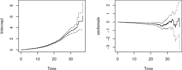
Obviously, sex is important; females have a lower mortality. Plots of the time-varying cumulative intercept and regression coefficient are given by
> oldpar <- par(mfrow = c(1, 2))
> plot(fit)
> par(oldpar)
See Figure 9.2, where 95% confidence limits are added around the fitted time-varying cumulative coefficients. Also note the use of the function par; the first call to it sets the plotting area to “one row and two columns” and saves the old par-setting in oldpar. Then the plotting area is restored to what it was earlier.
9.5 Dynamic Path Analysis
The term dynamic path analysis is coined by Odd Aalen and coworkers (Aalen et al. 2008). It is an extension, by explicitly introducing time, of path analysis described by (Wright 1921).
The inclusion of time in the model implies that there are one path analysis at each time point; see Figure 9.3.
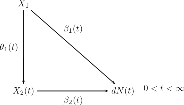
Dynamic path analysis; X2 is an intermediate covariate, while X1 is measured at baseline (t = 0). dN(t) is the number of events at t.
The structural equations
are estimated by ordinary least squares (linear regression) at each t with dN(t) > 0. Then the second equation is inserted in the first:
and the total treatment effect is (β1(t) + θ1(t)β2(t))dt, so it can be split into two parts according to
Some book-keeping is necessary in order to write an R function for this dynamic model. Of great help is the function risksets in eha; it keeps track of the composition of the riskset over time, which is exactly what is needed for implementing the dynamic path analysis.
9.6 Matching
Matching is a way of eliminating the effect of confounders and therefore important to discuss in connection with causality. One reason for matching is the wish to follow the causal inference paradigm with counterfactuals. Another reason is that the exposure we want to study is very rare in the population. It will then be inefficient to take a simple random sample from the population; in order to get enough cases in the sample, the sample size needs to be very large. On the other hand, today’s register-based research tends to analyze whole populations, and the limitations in terms of computer memory and processing power are more or less gone. Nevertheless, small, properly matched data sets may contain more information about the specific question at hand than a standard regression analysis on the whole register!
When creating a matched data set, we have to decide how many controls we want per case. In the true counterfactual paradigm in “causal inference,” it is common practice to choose one control per case, to “fill in” the unobservable in the pair of counterfactuals. We first look at the case with matched pairs, then a case study with two controls per case.
9.6.1 Paired Data
Certain kinds of observations come naturally in pairs. The most obvious situation is data from twin studies. Many countries keep registers of twins, and the advantage with twin data is that it is possible to control for genetic variation; monozygotic twins have identical genes. Humans have pairs of many details: arms, legs, eyes, ears, etc. This can be utilized in medical studies concerning comparison of treatments, the two in a pair simply get one treatment each.
In a survival analysis context, pairs are followed over time and it is noted who first experiencesthe event of interest. In each pair, one is treated and the other is a control, but otherwise they are considered more or less identical. Right censoring may make it impossible to decide who in the pair experienced the event first. Such pairs are simply discarded in the analysis.
The model is
where x is treatment (0-1) and i is the pair No. Note that each pair has its own baseline hazard function, which means that the proportional hazards assumption is only required within pairs. This is a special form of stratified analysis in that each stratum only contains two individuals, a case and its control. If we denote by Ti1 the life length of the case in pair No. i and Ti0 the life length of the corresponding control, we get
and the result of the analysis is simply a study of binomial data; how many times did the case die before the control? We can estimate this probability, and also test the null hypothesis that it is equal to one half, which corresponds to β = 0 in (9.1).
9.6.2 More than One Control
The situation with more than one control per case is as simple as the paired data case to handle. Simply stratify, with one case and its controls per stratum. It is also possible to have a varying number of controls per case.
As an example where two controls per case were used, let us see how a study of maternal death and its effect on infant mortality was performed (Broström 1987).
Example 30 Maternal death and infant mortality.
This is a study on historical data from northern Sweden, 1820–1895 (Broström 1987). The simple question asked was: How much does the death risk increase for an infant that loses her mother? More precisely, by a maternal death we mean that a mother dies within one year after the birth of her child. In this particular study, only first births were studied. The total number of such births was 5,641 and of these 35 resulted in a maternal death (with the infant still alive). Instead of analyzing the full data set, it was decided to use matching. To each case of maternal death, two controls were selected in the following way. At each time an infant changed status from mother alive to mother dead, two controls are selected without replacement from the subset of the current risk set, where all infants have mother alive and not already used as controls and with correct matching characteristics. If a control changes status to case (its mother dies), it is immediately censored as a control and starts as a case with two controls linked to it. However, this situation never occurred in the study.
Let us load the data into R and look at it.
> require(eha)
> data(infants)
> head(infants)
stratum enter exit event mother age sex parish civst
1 1 55 365 0 dead 26 boy Nedertornea married
2 1 55 365 0 alive 26 boy Nedertornea married
3 1 55 365 0 alive 26 boy Nedertornea married
4 2 13 76 1 dead 23 girl Nedertornea married
5 2 13 365 0 alive 23 girl Nedertornea married
6 2 13 365 0 alive 23 girl Nedertornea married
ses year
1 farmer 1877
2 farmer 1870
3 farmer 1882
4 other 1847
5 other 1847
6 other 1848
Here, we see the two first triplets in the data set, which consists of 35 triplets, or 105 individuals. Infant No. 1 (the first row) is a case, his mother died when he was 55 days old. At that moment, two controls were selected, that is, two boys 55 days of age, and with the same characteristics as the case. The matching was not completely successful; we had to look a few years back and forth in calendar time (covariate year). Note also that in this triplet all infants survived one year of age, so there is no information of risk differences in it. It will be automatically removed in the analysis.
The second triplet, on the other hand, will be used, because the case dies at age 76 days, while both controls survive one year of age. This is information suggesting that cases have higher mortality than controls after the fatal event of a maternal death.
The matched data analysis is performed by stratifying on triplets (the variable stratum).
> fit <- coxreg(Surv(enter, exit, event) ˜ mother + strata(stratum),
data = infants)
> fit
Call:
coxreg(formula = Surv(enter, exit, event) ˜ mother + strata(stratum),
data = infants)
Covariate Mean Coef Rel.Risk S.E. Wald p
mother
alive 0.763 0 1 (reference)
dead 0.237 2.605 13.534 0.757 0.001
Events 21
Total time at risk 21616
Max. log. likelihood -10.815
LR test statistic 19.6
Degrees of freedom 1
Overall p-value 9.31744e-06
The result is that the mother’s death increases the death risk of the infant by a factor 13.5! It is statistically very significant, but the number of infant deaths (21) is very small, so the p-value may be unreliable. A note in passing: The “Overall p-value” is the likelihood ratio test p-value for the whole model versus a model with no covariates. Since in this case there is only one regression parameter to estimate, the “Wald p” and the “Overall p-value” corresponds to the same null hypothesis, “mother’s death has no effect on her infant’s survival chances.” The part “e-06” means “move the decimal point six steps to the left,” giving the value 0.00000931744 ≈ 0.00001. Normally, this is the p-value to trust; see the discussion of the Hauck–Donner effect in Appendix A.
In a stratified analysis, it is normally not possible to include covariates that are constant within strata. However, here it is possible to estimate the interaction between a stratum-constant covariate and exposure, that is, mother’s death. However, it is important not to include the main effect corresponding to the stratum-constant covariate! This is a rare exception to the rule that when an interaction term is present, the corresponding main effects must be included in the model.
We investigate whether the effect of mother’s death is modified by her age by first calculating an interaction term (mage):
> infants$mage <- ifelse(infants$mother == “dead”, infants$age, 0)
Note the use of the function ifelse: It takes three arguments; the first is a logical expression (resulting in a logical vector, with values TRUE and FALSE. Note that in this example, the length is the same as the length of mother (in infants). For each component that is TRUE, the result is given by the second argument, and for each component that is FALSE the value is given by the third argument.
Including the created covariate in the analysis gives
> fit <- coxreg(Surv(enter, exit, event) ˜ mother + mage +
strata(stratum), data = infants)
> fit
Call:
coxreg(formula = Surv(enter, exit, event) ˜ mother + mage +
strata(stratum), data = infants)
Covariate Mean Coef Rel.Risk S.E. Wald p
mother
alive 0.763 0 1 (reference)
dead 0.237 2.916 18.467 4.860 0.548
mage 6.684 -0.012 0.988 0.188 0.948
Events 21
Total timeatrisk 21616
Max. log. likelihood -10.813
LR test statistic 19.6
Degreesoffreedom 2
Overall p-value 5.40649e-05
What happened here? The effect of the mother’s age is even larger than in the case without mage, but the statistical significance has vanished altogether. There are two problems with one solution here. First, due to the inclusion of the interaction, the (main) effect of mother’s death is now measured at the mother’s age equal to 0 (zero!), which of course is completely nonsensical, and second, the construction makes the two covariates strongly correlated: When mother is alive mage is zero, and when mother is dead, mage takes a rather large value. This is a case of collinearity, however, not a very severe case, because it is very easy to get rid of.
The solution to both problems is to center the mother’s age (age)! Recreate the variables and run the analysis again:
> infants$age <- infants$age - mean(infants$age)
> infants$mage <- ifelse(infants$mother == “dead”, infants$age, 0)
> fit1 <- coxreg(Surv(enter, exit, event) ˜ mother + mage +
strata(stratum), data = infants)
> fit1
Call:
coxreg(formula = Surv(enter, exit, event) ˜ mother + mage +
strata(stratum), data = infants)
Covariate Mean Coef Rel.Risk S.E. Wald p
mother
alive 0.763 0 1 (reference)
dead 0.237 2.586 13.274 0.809 0.001
mage 0.280 -0.012 0.988 0.188 0.948
Events 21
Total time at risk 21616
Max. log. likelihood -10.813
LR test statistic 19.6
Degrees of freedom 2
Overall p-value 5.40649e-05
The two fits are equivalent (look at the Max. log. likelihoods), but with different parametrizations. The second, with a centered mother’s age, is preferred, because the two covariates are close to uncorrelated there.
A subject-matter conclusion in any case is that the mother’s age does not affect the effect of her death on the survival chances of her infant.
A general advice: Always center continuous covariates before the analysis! This is especially important in the presence of models with interaction terms, and the advice is valid for all kinds of regression analyses, not only Cox regression.
9.7 Conclusion
Finally, some thoughts about causality, and the techniques in use for “causal inference.” As mentioned above, in order to claim causality, one must show (or assume) that there are “no unmeasured confounders.” Unfortunately, this is impossible to prove or show from data alone, but even worse is the fact that in practice, at least in demographic and epidemiological applications, there are always unmeasured confounders present. However, with this in mind, note that
Causal thinking is important.
Counterfactual reasoning and marginal models yield little insight into “how it works,” but it is a way of reasoning around research problems that helps sorting out thoughts.
- – Joint modeling is the alternative.
Creation of pseudo-populations through weighting and matching may limit the understanding of how things work.
- – Analyze the process as it presents itself, so that it is easier to generalize findings.
Read more about this in Aalen et al. (2008).