Appendix C

A Brief Introduction to R

There are already many excellent sources of information available for those who want to learn more about R. A visit to the R home page, http:\www.r-project.org, is highly recommendable. Look under Documentation. When R is installed on a computer, it is easy to access the documentation that comes with the distribution; start R and open the html help (?help.start). A good start for a beginner is also the book Introductory Statistics with R by Dalgaard (2008). The book on S Programming by Venables & Ripley (2000) is recommended for the more advanced studies of the topic that its title implies.

C.1 R in General

In this section we investigate how to work with R in general, without special reference to event history analysis, which will be treated separately in a later section in this chapter.

C.1.1 R Objects

R is an object-oriented programming language, which have certain implications for terminology. So is for instance everything i R objects. We will not draw too much on this fact, but it may be useful to know.

C.1.2 Expressions and Assignments

Commands are either expressions or assignments. Commands are separated by newline (normally) or semicolon. The hash mark (#) marks the rest of the line as a comment.

> 1 + exp(2.3) # exp is the exponential function

[1] 10.97418

> x <- 1 + exp(2.3)

> x

[1] 10.97418

Note that the R prompt is >. If the previous expression is incomplete, it changes to +.

The first line above is an expression. It is evaluated as return is pressed, and the result is normally printed. The second line is an assignment; the result is stored in x and not printed. By typing x, its content is normally printed.

The assignment symbol is “<-”, which consists of two consecutive key strokes, “<” followed by “-”. It is strongly recommended to enclose the assignment symbol (and any arithmetic operator) between spaces. It is forbidden to separate the two symbols by a space! You will then get comparison with something negative:

> x <- 3

> x < - 3

[1] FALSE

C.1.3 Objects

Everything in R is an object (object-oriented programming). All objects have a mode and a length. Data objects have modes numeric, complex, logical, or character, and language objects have modes function, call, expression, name, etc. All data objects are vectors; there are no scalars in R.

Vectors contain elements of the same kind; a list can be thought of as a vector where each element can be anything, even a list, and the elements can be completely different.

There are more properties of objects worth mentioning, but we save that for the situations where we need them.

C.1.4 Vectors and Matrices

There are five basic types of vectors: logical, integer, double, complex, and character. The function c (for concatenate) creates vectors:

> dat <- c(2.0, 3.4, 5.6)

> cols <- c(“red”, “green”, “blue”)

The elements of a vector may be named:

> names(dat) <- c(“Sam”, “John”, “Kate”)

> names(dat)

[1] “Sam” “John” “Kate”

> dat

 Sam John Kate

 2.0 3.4 5.6

> dat[“John”]

John

 3.4

Note the first two lines; names may either display (second row) or replace (first row).

The function matrix creates a matrix (surprise!):

> Y <- matrix(c(1,2,3,4,5,6), nrow = 2, ncol = 3)

> Y

 [,1] [,2] [,3]

[1,] 1 3 5

[2,] 2 4 6

> dim(Y) <- c(3, 2)

> Y

 [,1] [,2]

[1,] 1 4

[2,] 2 5

[3,] 3 6

> as.vector(Y)

[1] 1 2 3 4 5 6

> mode(Y)

[1] “numeric”

> attributes(Y)

$dim

[1] 3 2

It is also possible to create vectors by the functions numeric, character, and logical.

> x <- logical(7)

> x

[1] FALSE FALSE FALSE FALSE FALSE FALSE FALSE

> x <- numeric(7)

> x

[1] 0 0 0 0 0 0 0

> x <- character(7)

> x

[1] ““ ”” ““ ”” ““ ”” “”

These functions are useful for allocating storage (memory), which later can be filled. This is better practise than letting a vector grow sequentially.

The functions nrow and ncol extracts the number of rows and columns, respectively, of a matrix.

An array is an extension of a matrix to more than two dimensions.

C.1.5 Lists

Family records may be produced as a list:

> fam <- list(FamilyID = 1, man = “John”, wife = “Kate”,

   children = c(“Sam”, “Bart”))

> fam

$FamilyID

[1] 1

$man

[1] “John”

$wife

[1] “Kate”

$children

[1] “Sam” “Bart”

> fam$children

[1] “Sam” “Bart”

C.1.6 Data Frames

A data frame is a special case of a list. It consists of variables of the same length, but not necessarily of the same type. Data frames are created by either data.frame or read.table, where the latter reads data from an ASCII file on disk.

> dat <- data.frame(name = c(“Homer”, “Flanders”, “Skinner”),

     income = c(1000, 23000, 85000))

> dat

  name income

1 Homer  1000

2 Flanders 23000

3 Skinner 85000

A data frame has row names (here: 1, 2, 3) and variable (column) names (here: name, income). The data frame is the normal unit for data storage and statistical analysis in R.

C.1.7 Factors

Categorical variables are conveniently stored as factors in R.

> country <- factor(c(“se”, “no”, “uk”, “uk”, “us”))

> country

[1] se no uk uk us

Levels: no se uk us

> print.default(country)

[1] 2 1 3 3 4

Factors are internally coded by integers (1, 2, ...). The levels are by default sorted into alphabetical order. Can be changed:

> country <- factor(c(“se”, “no”, “uk”, “uk”, “us”),

     levels = c(“uk”, “us”, “se”, “no”))

> country

[1] se no uk uk us

Levels : uk us se no

The first level often have a special meaning (“reference category”) in statistical analyses in R. The function relevel can be used to change the reference category for a given factor.

C.1.8 Operators

Arithmetic operations are performed on vectors, element by element. The common operators are + - * / ^, where ^ is exponentiation. For instance,

> x <- c(1, 2, 3)

> x^2

[1] 1 4 9

> y <- 2 * x

> y / x

[1] 2 2 2

C.1.9 Recycling

The last examples above were examples of recycling; If two vectors of different lengths occur in an expression, the shorter one is recycled (repeated) as many times as necessary. For instance,

> x <- c(1, 2, 3)

> y <- c(2, 3)

> x / y

[1] 0.5000000 0.6666667 1.5000000

Warning message:

In x/y : longer object length is not a multiple of shorter object

length

so the actual operation performed is

> c(1, 2, 3) / c(2, 3, 2) # Truncated to equal length

[1] 0.5000000 0.6666667 1.5000000

It is most common with the shorter vector being of length one, that is, a scalar multiplication. If the length of the longer vector is not a multiple of the length of the shorter vector, a warning is issued; see output above. This is often a sign of a mistake in the code.

C.1.10 Precedence

Multiplication and division is performed before addition and subtraction, as in pure mathematics. The (almost) full set of rules is displayed in Table C.1.

It is, however, highly recommended to use parentheses often rather than relying on remembering those rules. Compare, for instance,

> 1:3 + 1

[1] 2 3 4

> 1:(3 + 1)

[1] 1 2 3 4

For descriptions of specific operators, consult the help system.

C.2 Some Standard R Functions

1. round, floor, ceiling: Rounds to nearest integer, downwards, and upwards, respectively.

   > round(2.5) # Round to even

   [1] 2

   > floor(2.5)

   [1] 2

   > ceiling(2.5)

   [1] 3

2. %/% and %% for integer divide and modulo reduction.

   > 5 %/% 2

   [1] 2

   > 5 %% 2

   [1] 1

3. Mathematical functions: abs, sign, log, exp, etc.

4. sum, prod, cumsum, cumprod for sums and products.

5. min, max, cummin, cummax for extreme values.

6. pmin, pmax parallel min and max.

   > x <- c(1, 2, 3)

   > y <- c(2, 1, 4)

   > max(x, y)

   [1] 4

   > pmax(x, y)

   [1] 2 2 4

7. sort, order for sorting and ordering. Especially useful is order for rearranging a data frame according to a specific ordering of one variable:

   > require(eha)

   > data(mort)

   > mt <- mort[order(mort$id, -mort$enter),]

   > last <- mt[!duplicated(mt$id),]

   First, mort is sorted after id, and within id decreasingly after enter (notice the minus sign in the formula!). Then all rows with duplicated id are removed, only the first appearance is kept. In this way we get a data frame with exactly one row per individual, the row that corresponds to the individual’s last (in age or calendar time). See the next item!

8. duplicated and unique for marking duplicated elements in a vector and removing duplicates, respectively.

   > x <- c(1,2,1)

   > duplicated(x)

   [1] FALSE FALSE TRUE

   > unique(x)

   [1] 1 2

   > x[!duplicated(x)]

   [1] 1 2

C.2.1 Sequences

The operator : is used to generate sequences of numbers.

> 1:5

[1] 1 2 3 4 5

> 5:1

[1] 5 4 3 2 1

> -1:5

[1] -1 0 1 2 3 4 5

> -(1:5)

[1] -1 -2 -3 -4 -5

> -1:-5

[1] -1 -2 -3 -4 -5

Don’t trust that you remember rules of precedence; use parentheses! There is also the functions seq and rep, see the help pages!

C.2.2 Logical expression

Logical expressions can take only two distinct values, TRUE and FALSE (note uppercase; R acknowledges the difference between lower case and upper case, unlike, e.g., Windows).

Logical vectors may be used in ordinary arithmetic, when they are coerced into numeric vectors with FALSE equal to zero and TRUE equal to one.

C.2.3 Indexing

Indexing is a powerful feature in R. It comes in several flavors.

A logical vector Must be of the same length as the vector it is applied to.

> x <- c(-1:4)

> x

[1] -1 0 1 2 3 4

> x[x > 0]

[1] 1 2 3 4

Positive integers Selects the corresponding values.

Negative integers Rejects the corresponding values.

Character strings For named vectors; select the elements with the given names.

Empty Selects all values. Often used to select rows/columns from a matrix,

> x <- matrix(c(1,2,3,4), nrow = 2)

> x

 [,1] [,2]

[1,] 1 3

[2,] 2 4

> x[, 1]

[1] 1 2

> x[, 1, drop = FALSE]

 [,1]

[1,] 1

[2,] 2

Note that a dimension is lost when one row/column is selected. This can be overridden by the argument drop = FALSE (don’t drop dimension(s)).

C.2.4 Vectors and Matrices

A matrix is a vector with a dim attribute.

> x <- 1:4

> x

[1] 1 2 3 4

> dim(x) <- c(2, 2)

> dim(x)

[1] 2 2

> x

 [,1] [,2]

[1,] 1 3

[2,] 2 4

> t(x)

 [,1] [,2]

[1,] 1 2

[2,] 3 4

Note that matrices are stored column-wise. The function t gives the transpose of a matrix.

An example of matrix multiplication.

> x <- matrix(c(1,2,3,4, 5, 6), nrow = 2)

> x

 [,1] [,2] [,3]

[1,] 1 3 5

[2,] 2 4 6

> y <- matrix(c(1,2,3,4, 5, 6), ncol = 2)

> y

 [,1] [,2]

[1,] 1 4

[2,] 2 5

[3,] 3 6

> y %*% x

 [,1] [,2] [,3]

[1,] 9  19  29

[2,]  12  26  40

[3,]  15  33  51

> x %*% y

 [,1] [,2]

[1,]  22  49

[2,]  28  64

Dimensions must match according to ordinary mathematical rules.

C.2.5 Conditional Execution

Conditional execution uses the if statement (but see also switch). Conditional constructs are typically used inside functions.

> x <- 3

> if (x > 3) {

  cat(“x is larger than 3
”)

 }else{

  cat(“x is smaller than or equal to 3
”)

 }

x is smaller than or equal to 3

See also the functions cat and print.

C.2.6 Loops

Loops are typically only used inside functions.

1. A for loop makes an expression to be iterated as a variable assumes all values in a sequence.

   > x <- 1

   > for (i in 1:4){

     x <- x + 1

     cat(“i = ”, i, “, x = ”, x, “
   ”)

    }

   i = 1 , x = 2

   i = 2 , x = 3

   i = 3 , x = 4

   i = 4 , x = 5

   > x

   [1] 5

2. The while loop iterates as long as a condition is TRUE.

   > done <- FALSE

   > i <- 0

   > while (!done & (i < 5)){

     i <- i + 1

     done <- (i > 3)

    }

   > if (!done) cat(“Did not converge
   ”)

3. The repeat loop iterates indefinitely or until a break statement is reached.

   > i <- 0

   > done <- FALSE

   > repeat{

     i <- i + 1

     done <- (i > 3)

     if (done) break

    }

   > i

   [1] 4

C.2.7 Vectorizing

In R, there is a family of functions that operates directly on vectors. See the documentation of apply, tapply, lapply, and sapply.

C.3 Writing Functions

Functions are created by assignment using the keyword function.

> fun <- function(x) exp(x)

> fun(1)

[1] 2.718282

This function, fun, is the exponential function, obviously. Usually, the function body consists of several statements.

> fun2 <- function(x, maxit){

  if (any(x <= 0)) error(“Only valid for positive x”)

  i <- 0

  sum <- 0

  for (i in 0:maxit){

   sum <- sum + x^i / gamma(i + 1)

 }

  sum

}

> fun2(1, 5)

[1] 2.716667

> fun2(1:5, 5)

[1] 2.716667 7.266667 18.400000 42.866667 91.416667

This function, fun2, uses the Taylor expansion of exp(x) for calculation. This is a very crude variant, and it is only good for positive x. It throws an error if fed by a negative value. Note that it is vectorized, that is, its first argument may be a real-valued vector. Also note the use of the function any.

In serious function writing, it is very unconvenient to define the function at the command prompt. It is much better to write it in a good editor and then source it into the R session as needed. If it will be used extensively in the future, the way to go is to write a package. This is covered in Writing R Extensions, available from the help system. Our favourite editor, and the one used in examples in these notes, is emacs, which is free and available on all platforms. Make sure you use ESS (Emacs Speaks Statistics) together with emacs. Emacs and ESS are easily found by searching the web.

Functions can be defined inside the body of another function. In this way, it is hidden for other functions, which is important when considering scoping rules. This is a feature that is not available in FORTRAN (77) or C. Suppose that the function inside is defined inside the function head.

1. The function inside is not visible outside head and cannot be used there.
2. A call to inside will use the function defined in head, and not some function outside with the same name.

The return value of a function is the value of the last expression in the function body.

C.3.1 Calling Conventions

The arguments to a function are either specified or unspecified (or both). Unspecified arguments are shown as “...” in the function definition. See, for instance, the functions c and min. The “...”may be replaced by any number of arguments in a call to the function.

The formal arguments are those specified in the function definition, and the actual arguments are those given in the actual call to the function. The rules by which formal and actual arguments are matched are

1. Any actual argument given as name = value, where name exactly matches a formal argument, is matched.
2. Arguments specified by name = value, but no exact match, are then considered. If a perfect partial match is found, it is accepted.
3. The remaining unnamed arguments are then matched in sequence (positional matching).
4. Remaining unmatced actual arguments are part of the ...argument if there is one. Otherwise, an error occurs.
5. Formal arguments need not be matched.

C.3.2 The Argument “...”

The purpose of the ... argument is usually to pass arguments to a function call inside the actual function. An example with the plot function, see Figure C.1:

> source(“dots.R”)

> dots

function (x, ...)

{

 plot(x, ...)

}

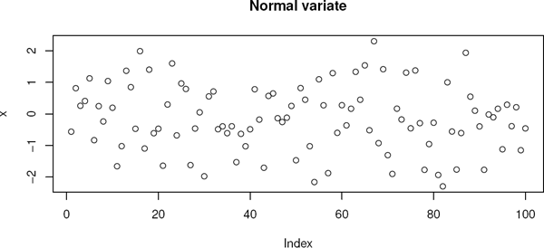
Note that “dot arguments” must be named in the function call.

C.3.3 Writing Functions

Below is a function that calculates the maximum likelihood estimate of the parameter in the exponential distribution, given a censored sample.

> source(“mlexp.R”)

> mlexp

function (x, d)

{

 n <- length(x)

 if (any(x <= 0))

   stop(“This function needs positive x”)

 if (length(d) != n)

   stop(“Lengths of x and d do not match”)

 d <- as.numeric(d != 0)

 sumx <- sum(x)

 sumd <- sum(d)

> dots(rnorm(100), main = “Normal variate”)

 loglik <- function(alpha) {

   sumd * alpha - sumx * exp(alpha)

}

 dloglik <- function(alpha) {

   sumd - sumx * exp(alpha)

}

 alpha <- 0

 res <- optim(alpha, fn = loglik, gr = dloglik, method = “BFGS”,

   control = list(fnscale = -1))

 res

}

First note that the arguments of the function, x and d, do not have any default values. Both arguments must be matched in the actual call to the function. Second, note the check of sanity in the beginning of the function and the calls to stop in case of an error. For less severe mistakes it is possible to give a warning, which does not break the execution of the function.

> exit <- rexp(100, 1)

> event <- as.numeric(exit < 2)

> exit <- pmax(exit, 2)

> res <- mlexp(exit, event)

> res $par

[1] -0.8450675

$value

[1] -166.0561

$counts

function gradient

  20   6

$convergence

[1] 0

$message

NULL

> unlist(res)

   par  value counts.function counts.gradient

 -0.8450675 -166.0560743  20.0000000  6.0000000

 convergence

  0.0000000

C.3.4 Lazy Evaluation

When a function is called, the arguments are parsed, but not evaluated until it is needed in the function. Specifically, if the function does not use the argument, it is never evaluated, and the variable need not even exist. This is in contrast to rules in C and FORTRAN.

> fu <- function(x, y) 2 * x

> fu(3)

[1] 6

> fu(3, y = zz)

[1] 6

> exists(“zz”)

[1] FALSE

C.3.5 Recursion

Functions are allowed to be recursive, that is, a function in R is allowed to call itself. As an example, the function gsort, defined below, does sorting by finding the smallest value in a vector to be sorted, and then calls itself on the remaining values after the smallest is removed.

> source(“gsort.R”)

> gsort

function (x)

{

 n <- length(x)

 if (n == 1)

   return(x)

 sorted <- numeric(n)

 smallest <- which.min(x)

 sorted[1] <- x[smallest]

 sorted[2:n] <- gsort(x[-smallest])

 sorted

}

> gsort(rnorm(10))

[1] -0.3147130 -0.1752400 0.1704180 0.2291849 0.4321751

[6] 0.4782381 1.2201831 1.2799731 1.3885228 1.3996963

Use this technique with extreme caution; it is extremely memory-intensive, and may be very slow. On the plus side is that it allows very neat algorithms.

More compact code:

> source(“gcsort.R”)

> gcsort

function (x)

{

 if (length(x) == 1)

   return(x)

 smallest <- which.min(x)

 c(x[smallest], gsort(x[-smallest]))

}

C.3.6 Vectorized Functions

Most mathematical functions in R are vectorized, meaning that if the argument to the function is a vector, then the result is a vector of the same length. Some functions apply the recycling rule to vectors shorter than the longest:

> sqrt(c(9, 4, 25))

[1] 3 2 5

> pnorm(1, mean = 0, sd = c(1,2,3))

[1] 0.8413447 0.6914625 0.6305587

When writing own functions, the question of making it vectorized should always be considered. Often, it is automatically vectorized, like

> fun <- function(x) 3 * x - 2

> fun(c(1,2,3))

[1] 1 4 7

but not always. Under some circumstances, it may be necessary to explicitly make the calculations separately for each element in a vector.

C.3.7 Scoping Rules

Within a function in R, objects are found in the following order:

1. It is a locally defined variable.
2. It is in the argument list.
3. It is defined in the environment where the function is defined.

> source(“scop.R”)

> scop

function (x)

{

 y <- x^2

 z <- 2

 fun <- function(p) {

   z <- 0

   m <- exp(p * y) + x - z

   m

}

 fun(z)

}

> scop(2)

[1] 2982.958

Note that a function will eventually look for the variable in the work space. This is often not the intention!

Tip: Test functions in a clean workspace. For instance, start R with the flag -vanilla.

C.4 Graphics

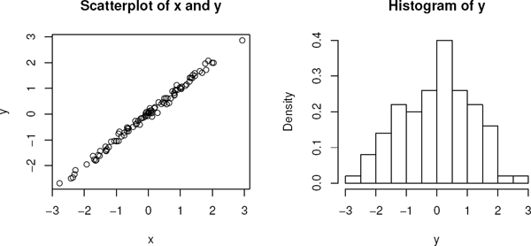
The workhorses in standard graphics handling in R are the functions plot and par. Read their respective documentations carefully; you can manipulate your plots almost without limitation!

See the code and Figure C.2 for the output.

> source(“plot2.R”)

> plot2

function ()

{

 x <- rnorm(100)

 y <- x + rnorm(100, sd = 0.1)

 oldpar <- par(mfrow = c(1, 2))

 on.exit(par(oldpar))

 plot(x, y, main = “Scatterplot of x and y”)

 hist(y, main = “Histogram of y”, probability = TRUE)

}

> plot2()

C.5 Probability Functions

In R several of the common distributions are represented by (at least) four functions each, one for density (prefix d), one for probability (prefix p), one for quantile (prefix q), and one for random number generation (prefix r). For a list of available functions and more detailed information about them, see Chapter 8 in An Introduction to R. See also the online help system, for instance,

> ?pnorm

Some special packages contain more distribtions, for instance, the eha package (extreme-value, Gompertz, piecewise constant hazard). See Appendix B for more detail.

C.5.1 Some Useful R Functions

C.5.1.1 Matching

There are some useful functions in R doing set operations. For exact definitions of these functions, see the documentation.

match match(x, y) returns a vector of the same length as x with the place of the first occurrence of each element in x in y. If there is mo match for a particular element in x, NA is returned (can be changed). Example

> x <- c(1,3,2,5)

> y <- c(3, 2, 4, 1, 3)

> match(x, y)

[1] 4 1 2 NA

The match function is useful picking information in one data frame and put it in another (or the same). As an example, look at the data frame oldmort.

> require(eha)

> data(oldmort)

> names(oldmort)

 [1] “id”   “enter” “exit”  “event”

 [5] “birthdate” “m.id”  “f.id”  “sex”

 [9] “civ”  “ses.50” “birthplace” “imr.birth”

[13] “region”

Note the variables id (id of current record) and m.id (id of the mother to the current). Some of the mothers are also subjects in this file, and if we in an analysis want to use mother’s birthplace as a covariate, we can get it from her record (if present; there will be many missing mothers). This is accomplished with match; creating a new variable m.birthplace (mother’s birthplace) is as simple as

> oldmort$m.birthplace <- with(oldmort,

       birthplace[match(m.id, id)])

The tricky part here is to get the order of the arguments to match right. Always check the result on a few records!

%in% Simple version of match. Returns a logical vector of the same length as x, see below.

> x %in% y

[1] TRUE TRUE TRUE FALSE

A simple and efficient way of selecting subsets of a certain kind, For instance, to select all cases with parity 1, 2, or 3, use

> data(fert)

> f13 <- fert[fert$parity %in% 1:3,]

This is the same as

> f13 <- fert[(fert$parity >= 1) & (fert$parity <= 3),]

Note that the parantheses in the last line are strictly unnecessary, but their presence increases readability and avoids stupid mistakes about precedence between operators. Use parentheses often!

subset Selects subsets of vectors, arrays, and data frames. See the help page.

tapply Applies a function to all subsets of a data frame (it is more general than that; see the help page). Together with match it is useful for creating new summary variables for clusters and sticking the values to each individual.

If we for all rows in the fert data frame want to add the age at first birth for the corresponding mother, we can do this as follows.

> data(fert)

> indx <- tapply(fert$id, fert$id)

> min.age <- tapply(fert$age, fert$id, min)

> fert$min.age <- min.age[indx]

Check this for yourself! And read the help pages for match and tapply carefully.

C.5.1.2 General utility functions

pmax, pmin Calculates the parallel max and min, respectively.

> x <- c(2, 3, 1, 7)

> y <- c(1, 2, 3)

> pmin(x, y)

[1] 1 2 1 1

> min(x, y)

[1] 1

ifelse A vectorized version of if.

> x <- rexp(6)

> d <- ifelse(x > 1, 0, 1)

> x

[1] 1.2775732 0.5135248 0.4508808 0.9722598 2.1630381 0.3899085

> d

[1] 0 1 1 1 0 1

C.6 Help in R

Besides all documentation that can be found on CRAN (http://cran.r-project.org), there is an extensive help system online in R. To start the general help system, type

> help.start()

at the prompt (or, find a corresponding menu item on a GUI system). Then a help window opens up with access to several FAQs, and all the packages that are installed.

For immediate help on a specific function you know the name of, type

> ?coxreg

If you only need to see the syntax and input arguments, use the function args:

> args(coxreg)

function (formula = formula(data), data = parent.frame(), weights,

 subset, t.offset, na.action = getOption(“na.action”),

 init = NULL, method = c(“efron”, “breslow”, “mppl”, “ml”),

 control = list(eps = 1e-08, maxiter = 25, trace = FALSE),

 singular.ok = TRUE, model = FALSE, center = TRUE, x = FALSE,

 y = TRUE, boot = FALSE, efrac = 0, geometric = FALSE, rs = NULL,

 frailty = NULL, max.survs = NULL)

NULL

C.7 Functions in eha and survival

Here some useful functions in eha are listed. In most cases the description is very sparse, and the reader is recommended to consult the help pages when more detail is wanted.

aftreg Fits accelerated failure time (AFT) models.

age.window Makes a “horizontal cut” in the Lexis diagram, that is, it selects a subset of a data set based on age. The data frame must contain three variables that can be input to the Surv function. The default names are enter, exit, and event. As an example,

> require(eha)

> data(oldmort)

> mort6070 <- age.window(oldmort, c(60, 70))

limits the study of old age mortality to the (exact) ages between 60 and 70, that is. from 60.000 up to and including 69.999 years of age.

For rectangular cuts in the Lexiz diagram, use both age.window and cal.window in succession. The order is unimportant.

cal.window Makes a “vertical cut” in the Lexis diagram, that is, it selects a subset of a data set based on calendar time. As an example,

> require(eha)

> data(oldmort)

> mort18601870 <- cal.window(oldmort, c(1860, 1870))

limits the study of old age mortality to the time period between 1860 and 1870, that is, from 1 January 1860 up to and including 31 December 1869.

For rectangular cuts in the Lexiz diagram, use both age.window and cal.window in succession. The order is unimportant.

cox.zph Tests the proportionality assumption on fits from coxreg and coxph.

coxreg Fits Cox proportional hazards model. It is a wrapper for coxph in case of simpler Cox regression models.

glmmML Fits clustered binary and count data regression models.

phreg Fits parametric proportional hazards models.

risksets Finds the members of each riskset at all event times.

C.7.1 Checking the Integrity of Survival Data

In data sources collected through reading and coding old printed handwritten sources, many opportunities for making errors occur. Therefore, it is important to have tools for detecting logical errors like people dying before they got married, of living at two places at the same time. In the sources used in this book, such errors occur in almost all data retrievals. It is important to say that this fact is not a sign of a bad job in the transfer of data from old churchbooks to digital data files. The case is almost always that the errors are present in the original source, and in the registration process no corrections of “obvious” mistakes by the priests are allowed; the digital files are supposed to be as close as possible to the original sources. These are the rules at the Demographic Database (DDB), Umeå University.

This means that the researcher has a responsibility to check her data for logical (and other) errors, and truthfully report how she handles these errors. In my own experience with data from the DDB, the relative frequency of errors varies between 1 and 5 per cent. In most cases it would not do much harm to simply delete erroneous records, but often the errors are “trivial,” and it seems easy to guess what the truth should be.

Example 33 Old Age Mortality

As an example of the kind of errors discussed above, we take a look at the original version of oldmort in eha. For survival data in “interval” form (enter, exit], it is important that enter is smaller than exit. For individuals with more than one record, the intervals are not allowed to overlap, and at most one of them is allowed to end with an event. Note that we are talking about survival data, so there are no repeated events “by design.”

The function check.surv in eha tries to do these kinds of checks and report back all individuals (“id”) that do not follow the rules.

> load(“olm.rda”)

> require(eha)

> errs <- with(olm, check.surv(enter, exit, event, id))

> errs

 [1] “785000980” “787000493” “790000498” “791001135” “792001121”

 [6] “794001225” “794001364” “794001398” “796000646” “797001175”

[11] “797001217” “798001203” “800001130” “801000743” “801001113”

[16] “801001210” “801001212” “802001136” “802001155” “802001202”

[21] “803000747” “804000717” “804001272” “804001354” “804001355”

[26] “804001532” “805001442” “806001143” “807000736” “807001214”

[31] “808000663” “810000704” “811000705” “812001454” “812001863”

[36] “813000613” “814000799” “815000885” “816000894” “817000949”

[41] “819001046”

> no.err <- length(errs)

So, 41 individuals have bad records. Let us look at some of them.

> badrecs <- olm[olm$id %in% errs,]

> dim(badrecs)

[1] 105 13

> badrecs[badrecs$id == errs[1],]

   id enter  exit event birthdate  m.id  f.id

283 785000980 74.427 75.917 FALSE 1785.573 743000229 747000387

284 785000980 75.525 87.917 FALSE 1785.573 743000229 747000387

285 785000980 87.917 88.306  TRUE 1785.573 743000229 747000387

  sex civ ses.50 birthplace imr.birth region

283  female married farmer parish 12.4183  rural

284  female  widow farmer parish 12.4183  rural

285  female  widow farmer parish 12.4183  rural

The error here is that the second interval (75.526, 87.927] starts before the first interval has ended. We also see that this is a married woman who became a widow in the second record.

In this case, I think that a simple correction saves the situation: Let the second interval begin where the first ends. The motivation for this choice is that the first interval apparently ends with the death of the woman’s husband. Death dates are usually reliable, so I believe more in them than in other dates.

Furthermore, the exact choice here will have very little impact on the analyses we are interested in. The length of the overlap is less than half a year, and this person will eventually have the wrong civil status for at most that amount of time.

It turns out that all“bad”individuals are of this type. Therefore, we“clean” the data set by running it through this function:

ger <- function(){

 require(eha)

 load(“olm.rda”)

 out <- check.surv(olm$enter, olm$exit, olm$event, olm$id)

 ko <- olm[olm$id %in% out,]

 ## ko is all records belonging to “bad individuals”

 ## Sort ko, by id, then by interval start, then by event

 ko <- ko[order(ko$id, ko$enter, -ko$event),]

 for (i in ko$id){# Go thru all ‘bad individuals’

   slup <- ko[ko$id == i, , drop = FALSE]

   ## Pick out their records

   n <- NROW(slup)

   if (n > 1){# Change them

   for (j in (2:n)){

    slup$enter[j] <- slup$exit[j-1]

  }

   ## And put them back:

   ko[ko$id == i,] <- slup

  }

}

 ## Finally, put ‘all bad’ back into place:

 om <- olm

 om[om$id %in% out,] <- ko

 ## Keep only records that start before they end:

 om <- om[om$enter < om$exit,]

 om

}

Read the comments, lines (or part of lines) starting with #. The output of this function, om, is the present data file oldmort in eha, with the errors corrected as indicated above.

Running the function.

> source(“ger.R”)

> om <- ger()

> left <- with(om, check.surv(enter, exit, event, id))

> left

[1] “794001225”

Still one bad. Let us take a look at that individual.

> om[om$id == left,]

   id enter  exit event birthdate m.id f.id sex

1168 794001225 65.162 68.650 FALSE 1794.838  NA  NA male

1169 794001225 68.650 85.162 FALSE 1794.838  NA  NA male

1171 794001225 78.652 85.162 FALSE 1794.838  NA  NA male

  civ ses.50 birthplace imr.birth region

1168 widow farmer parish 12.70903  rural

1169 widow farmer region 12.70903  rural

1171 widow farmer parish 12.70903  rural

It seems as if this error (second an third records overlap) should have been fixed by our function ger. However, there may have been a record removed, so we have to look at the original data file:

> olm[olm$id == left,]

   id enter  exit event birthdate m.id f.id sex

1168 794001225 65.162 68.650 FALSE 1794.838  NA  NA male

1169 794001225 65.162 85.162 FALSE 1794.838  NA  NA male

1170 794001225 68.650 78.652 FALSE 1794.838  NA  NA male

1171 794001225 78.652 85.162 FALSE 1794.838  NA  NA male

  civ ses.50 birthplace imr.birth region

1168 widow farmer parish 12.70903  rural

1169 widow farmer region 12.70903  rural

1170 widow farmer parish 12.70903  rural

1171 widow farmer parish 12.70903  rural

Yes, after correction, the third record was removed. The matter can now be fixed through removing the last record in om[om$id == left,] :

> who <- which(om$id == left)

> who

[1] 1166 1167 1168

> om <- om[-who[length(who)],]

> om[om$id == left,]

   id enter  exit event birthdate m.id f.id sex

1168 794001225 65.162 68.650 FALSE 1794.838  NA  NA male

1169 794001225 68.650 85.162 FALSE 1794.838  NA  NA male

  civ ses.50 birthplace imr.birth region

1168 widow farmer parish 12.70903  rural

1169 widow farmer region 12.70903  rural

And we are done.

C.8 Reading Data into R

The first thing you have to do in a statistical analysis (in R) is to get data into the computing environment. Data may come from different kind of sources, and R has the capacity to read from many kinds of sources, like data files from other statistical programs, spreadsheet type (e.g., Excel) data. This is done with the aid of the package foreign.

If anything else fails, it is almost always possible to get data written in ASCII format (e.g., .csv files). These can be read into R with the function read.table, see the next section.

C.8.1 Reading Data from ASCII Files

Ordinary text (ASCII) files in tabular form can be read into R with the function read.table. For instance, with a file looking this:

enter exit event

 1 5 1

 2 7 1

 1 5 1

 0 6 0

we read it into R with

> mydata <- read.table(“my.dat”, header = TRUE)

Note the argument header. It can take two values, TRUE or FALSE, with FALSE being the default value. If header = TRUE, then the first row of the data file is interpreted as variable names.

There are a few optional arguments to read.table that are important to consider. The first is dec, which gives the character used as a decimal point. The default is “.”, but in some locales “,” (e.g., Swedish) is commonly used in output from other software than R. The second is sep, which gives the field separator character. The default value is ′′′′, which means “white space” (tabs, spaces, newlines, etc.). See the help page for all the possibilities, including the functions read.csv, read.csv2, etc., which are variations of read.table with other default values.

The result should always be checked after reading. Do that by printing a few rows

> head(mydata)

 enter exit event

1 1 5 1

2 2 7 1

3 1 5 1

4 0 6 0

and/or by summarizing the columns

> summary(mydata)

 enter  exit   event

Min.  :0.00 Min.  :5.00 Min.  :0.00

1st Qu.:0.75 1st Qu.:5.00 1st Qu.:0.75

Median :1.00 Median :5.50 Median :1.00

Mean  :1.00 Mean  :5.75 Mean  :0.75

3rd Qu.:1.25 3rd Qu.:6.25 3rd Qu.:1.00

Max.  :2.00 Max.  :7.00 Max.  :1.00

The str function is also helpful:

> str(mydata)

‘data.frame’:  4 obs. of 3 variables:

$ enter: int 1 2 1 0

$ exit : int 5 7 5 6

$ event: int 1 1 1 0

For each variable, its name and type is given, together with the first few values. In this example, it is all the values, and we can also see that R interprets all the values as integer. This is fine, even though at least enter and exit probably are supposed to be real-valued. In fact, R is not so strict with numerical types (as opposed to C and FORTRAN). Frequent coercing takes place, and the mode numeric contains the types integer and double.

Now this tends to be confusing, but the bottom line is that you, as a user, need not worry at all. Except in one place: When you are writing an R function that calls compiled C or FORTRAN code, but that is far beyond the scope of this book. Interested readers are recommended to read Venables & Ripley (2000).

C.8.2 Reading Foreign Data Files

Data file from MINITAB, SAS, SPSS, Stata, etc., can be read with a suitable function from the foreign package. Consult its help pages for more information.

The package Hmisc (Harrell Jr. 2011) contains some useful functions for reading data from foreign programs. They are usually wrappers for selected functions in the foreign package, but with convenient default behaviour.