2. Creating a Basic Pivot Table
In This Chapter
Preparing Data for Pivot Table Reporting
How to Create a Basic Pivot Table
Understanding the Recommended Pivot Table Feature
Keeping Up with Changes in the Data Source
Saving Time with New Pivot Table Tools
Preparing Data for Pivot Table Reporting
When you have a family portrait taken, the photographer takes time to make sure that the lighting is right, the poses are natural, and everyone smiles his or her best smile. This preparation ensures that the resulting photo is effective in its purpose.
When you create a pivot table report, you’re the photographer, taking a snapshot of your data. By taking time to make sure your data looks its best, you can ensure that your pivot table report is effective in accomplishing the task at hand.
One of the benefits of working in a spreadsheet is that you have the flexibility of laying out your data to suit your needs. Indeed, the layout you choose depends heavily on the task at hand. However, many of the data layouts used for presentations are not appropriate when used as the source data for a pivot table report.
Tip
As you read the following pages, which discuss preparing your data, keep in mind that pivot tables have only one hard rule pertaining to the data source: The data source must have column headings, which are labels in the first row of the data that describe the information in each column. Without column headings, you cannot create a pivot table report.
However, just because a pivot table report is created successfully does not mean that it’s effective. A host of things can go wrong as a result of bad data preparation—from inaccurate reporting to problems with grouping and sorting.
Let’s look at a few of the steps you can take to ensure that you end up with a viable pivot table report.
Ensuring That Data Is in a Tabular Layout
A perfect layout for the source data in a pivot table is a tabular layout. In tabular layout, there are no blank rows or columns. Every column has a heading. Every field has a value in every row. Columns do not contain repeating groups of data.
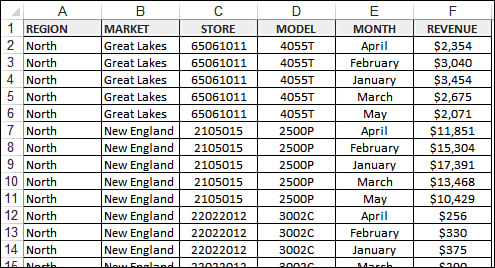
Figure 2.1 shows an example of data structured properly for a pivot table. There are headings for each column. Even though the values in D2:D6 are all the same model, the model number appears in each cell. Month data is organized down the page instead of across the columns.
Tabular layouts are database centric, meaning you would most commonly find these types of layouts in databases. These layouts are designed to store and maintain large amounts of data in a well-structured, scalable format.
Tip
You might work for a manager who demands that the column labels be split into two rows. For example, he might want the heading Gross Margin to be split, with Gross in row 1 and Margin in row 2. Because pivot tables require a unique heading one row high, your manager’s preference can be problematic. To overcome this problem, start typing your heading; for example, type Gross. Before leaving the cell, press Alt+Enter and then type Margin. The result is a single cell that contains two lines of data.
Avoiding Storing Data in Section Headings
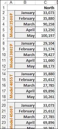
Examine the data in Figure 2.2. This spreadsheet shows a report of sales by month and model for the North region of a company. Because the data in rows 2 through 24 pertains to the North region, the author of the worksheet entered the title North as a single cell in C1. This approach is effective for display of the data, but it’s not effective for a pivot table data source.
Also in Figure 2.2, the author was very creative with the model information. The data in rows 2 through 6 applies to Model 2500P, so the author entered this value once in A2 and then applied a fancy vertical format combined with Merge Cells to create an interesting look for the report. Again, although this is a cool format, it is not useful for pivot table reporting.
Also, the worksheet in Figure 2.2 is missing column headings. You can guess that column A is Model, column B is Month, and column C is Sales, but for Excel to create a pivot table, this information must be included in the first row of the data.
Avoiding Repeating Groups as Columns
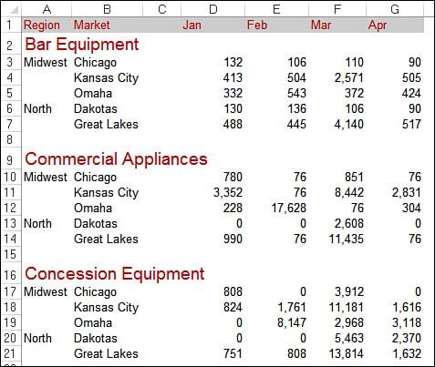
The format shown in Figure 2.3 is common. A time dimension is presented across several columns. Although it is possible to create a pivot table from this data, this format is not ideal.
Figure 2.3 This matrix format is common but not effective for pivot tables. The Month field is spread across several columns of the report.
The problem is that the headings spread across the top of the table pull double duty as column labels and actual data values. In a pivot table, this format would force you to manage and maintain six fields, each representing a different month.
Eliminating Gaps and Blank Cells in the Data Source
Delete all empty columns within your data source. An empty column in the middle of your data source causes your pivot table to fail on creation because the blank column, in most cases, does not have a column name.
Delete all empty rows within your data source. Empty rows may cause you to inadvertently leave out a large portion of your data range, making your pivot table report incomplete.
Fill in as many blank cells in your data source as possible. Although filling in cells is not required to create a workable pivot table, blank cells are generally errors waiting to happen. So a good practice is to represent missing values with some logical missing value code wherever possible.
Note
Although eliminating gaps and blank cells might seem like a step backward for those of you who are trying to create a nicely formatted report, it pays off in the end. When you are able to create a pivot table, there will be plenty of opportunities to apply some pleasant formatting.
Note
In Chapter 3, “Customizing a Pivot Table,” you’ll discover how to apply styles formatting to your pivot tables.
Applying Appropriate Type Formatting to Fields
Formatting fields appropriately helps you avoid a whole host of possible issues, from inaccurate reporting to problems with grouping and sorting.
Make certain that any fields to be used in calculations are explicitly formatted as a number, currency, or any other format appropriate for use in mathematical functions. Fields containing dates should also be formatted as any one of the available date formats.
Summary of Good Data Source Design
The attributes of an effective tabular design are as follows:
![]() The first row of your data source is made up of field labels or headings that describe the information in each column.
The first row of your data source is made up of field labels or headings that describe the information in each column.
![]() Each column in your data source represents a unique category of data.
Each column in your data source represents a unique category of data.
![]() Each row in your data source represents individual items in each column.
Each row in your data source represents individual items in each column.
![]() None of the column names in your data source double as data items that will be used as filters or query criteria (that is, names of months, dates, years, names of locations, or names of employees).
None of the column names in your data source double as data items that will be used as filters or query criteria (that is, names of months, dates, years, names of locations, or names of employees).
How to Create a Basic Pivot Table
Now that you have a good understanding of the importance of a well-structured data source, let’s walk through creating a basic pivot table.
Note
The sample data set used throughout this book is available for download at www.mrexcel.com/pivotbookdata2016.html.
To ensure that the pivot table captures the range of your data source by default, click any single cell in your data source. Next, select the Insert tab and find the Tables group. In the Tables group, select PivotTable and then choose PivotTable from the drop-down list. Figure 2.6 demonstrates how to start a pivot table.
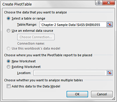
Choosing these options activates the Create PivotTable dialog, shown in Figure 2.7.
Tip
You can also press the shortcut Alt+N+V to start a pivot table.
As you can see in Figure 2.7, the Create PivotTable dialog asks you only two fundamental questions: Where’s the data that you want to analyze? and Where do you want to put the pivot table? Here’s how you handle these two sections of the dialog:
![]() Choose the Data That You Want to Analyze—In this section, you tell Excel where your data set is. You can specify a data set that is located within your workbook, or you can tell Excel to look for an external data set. As you can see in Figure 2.7, Excel is smart enough to read your data set and fill in the range for you. However, you always should take note of the range Excel selects to ensure that you are capturing all your data.
Choose the Data That You Want to Analyze—In this section, you tell Excel where your data set is. You can specify a data set that is located within your workbook, or you can tell Excel to look for an external data set. As you can see in Figure 2.7, Excel is smart enough to read your data set and fill in the range for you. However, you always should take note of the range Excel selects to ensure that you are capturing all your data.
![]() Choose Where You Want the PivotTable Report to Be Placed—In this section, you tell Excel where you want your pivot table to be placed. This is set to New Worksheet by default, meaning that your pivot table will be placed in a new worksheet within the current workbook. You will rarely change this setting because there are relatively few times you’ll need your pivot table to be placed in a specific location.
Choose Where You Want the PivotTable Report to Be Placed—In this section, you tell Excel where you want your pivot table to be placed. This is set to New Worksheet by default, meaning that your pivot table will be placed in a new worksheet within the current workbook. You will rarely change this setting because there are relatively few times you’ll need your pivot table to be placed in a specific location.
Note
Note the presence of another option in the Create PivotTable dialog shown in Figure 2.7: the Add This Data to the Data Model option. You would select this option if you were trying to consolidate multiple data sources into one single pivot table.
The Add This Data to the Data Model option is covered this option in detail in Chapter 7, “Analyzing Disparate Data Sources with Pivot Tables,” and in Chapter 10, “Mashing Up Data with Power Pivot.”
In this chapter, we’ll keep it basic by covering the steps to create a pivot table from using a single source, which means you can ignore this particular option.
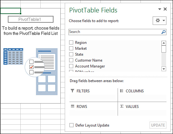
After you have answered the two questions in the Create PivotTable dialog, simply click the OK button. At this point, Excel adds a new worksheet that contains an empty pivot table report. Next to that is the PivotTable Fields list, shown in Figure 2.8. This pane helps you build your pivot table.
Adding Fields to a Report
You can add the fields you need to a pivot table by using the four “areas” found in the PivotTable Fields list: Filters, Columns, Rows, and Values. These areas, which correspond to the four areas of the pivot table, are used to populate your pivot table with data:
Note
Review Chapter 1, “Pivot Table Fundamentals,” for a refresher on the four areas of a pivot table.
![]() Filters—Adding a field to the Filters area enables you to filter on its unique data items. In previous versions of Excel, this area was known as the Report Filters area.
Filters—Adding a field to the Filters area enables you to filter on its unique data items. In previous versions of Excel, this area was known as the Report Filters area.
![]() Columns—Adding a field into the Columns area displays the unique values from that field across the top of the pivot table.
Columns—Adding a field into the Columns area displays the unique values from that field across the top of the pivot table.
![]() Rows—Adding a field into the Rows area displays the unique values from that field down the left side of the pivot table.
Rows—Adding a field into the Rows area displays the unique values from that field down the left side of the pivot table.
![]() Values—Adding a field into the Values area includes that field in the values area of your pivot table, allowing you to perform a specified calculation using the values in the field.
Values—Adding a field into the Values area includes that field in the values area of your pivot table, allowing you to perform a specified calculation using the values in the field.
Fundamentals of Laying Out a Pivot Table Report
Now let’s pause a moment and go over some fundamentals of laying out a pivot table report. This is generally the point where most new users get stuck. How do you know which field goes where?
Before you start dropping fields into the various areas, answer two questions: “What am I measuring?” and “How do I want to see it?” The answer to the first question tells you which fields in your data source you need to work with, and the answer to the second question tells you where to place the fields.
Say that in this case, you want to measure the dollar sales by region. This automatically tells you that you need to work with the Sale Amount field and the Region field. How do you want to see it? You want regions to go down the left side of the report and the sales amount to be calculated next to each region.
To achieve this effect, you need to add the Region field to the Rows area and add the Sale Amount field to the Values area.
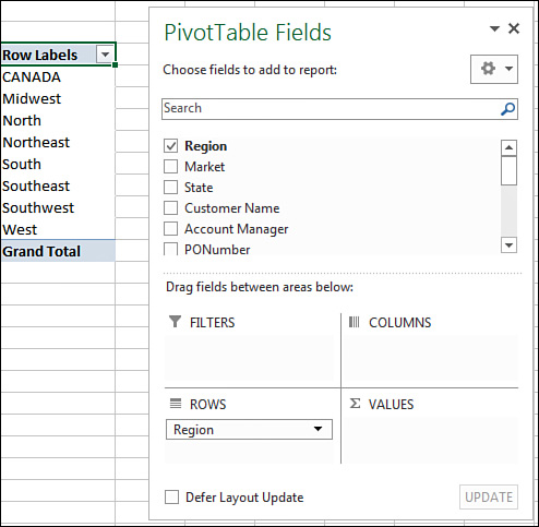
Find the Region field in the PivotTable Fields list, and place a check in the check box next to it. As you can see in Figure 2.9, not only is the field automatically added to the Rows area, but your pivot table is updated to show the unique region names.
Figure 2.9 Place a check next to the Region field to automatically add that field to your pivot table.
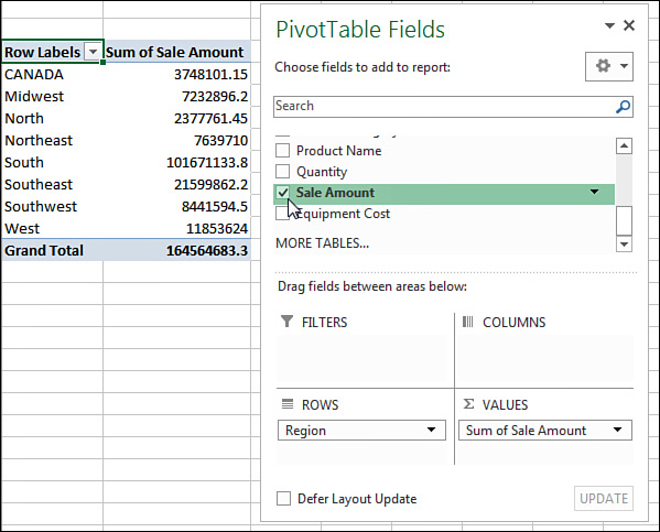
Now that you have regions in your pivot table, it’s time to add in the dollar sales. To do that, simply find the Sale Amount field and place a check next to it. As Figure 2.10 illustrates, the Sale Amount field is automatically added to the Values area, and your pivot table report now shows the total dollar sales for each region.
At this point, you have already created your first pivot table report!
Caution
Watch out for blanks in your numeric fields. If you have even one blank cell in a numeric field, Excel reads that cell as a Text field and therefore places it in the Rows area!
Adding Layers to a Pivot Table
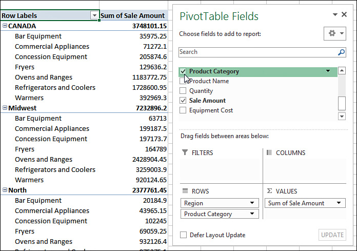
Now you can add another layer of analysis to your report. Say that now you want to measure the amount of dollar sales each region earned by product category. Because your pivot table already contains the Region and Sales Amount fields, all you have to do is place a check next to the Product Category field. As you can see in Figure 2.11, your pivot table automatically added a layer for Product Category and refreshed the calculations to include subtotals for each region. Because the data is stored efficiently in the pivot cache, this change took less than a second.
Figure 2.11 Without pivot tables, adding layers to analyses requires hours of work and complex formulas.
Rearranging a Pivot Table
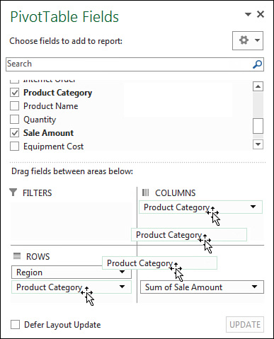
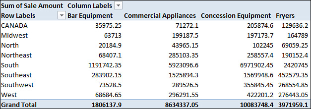
Suppose that the view you’ve created doesn’t work for your manager. He wants to see Product Categories across the top of the pivot table report. To make this change, simply drag the Product Category field from the Rows area to the Columns area, as illustrated in Figure 2.12.
You don’t have to move your fields into an area to be able to drag them around. You can actually drag fields directly from the list of fields in the PivotTable Fields list to the desired area. You can also move a field into an area by using that field’s context menu: Click the black triangle next to the field name and then select the desired area.
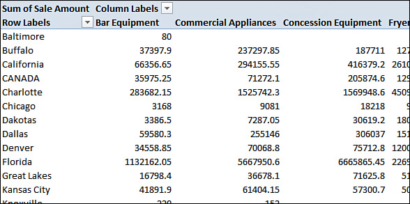
The report is instantly restructured, as shown in Figure 2.13.
Creating a Report Filter
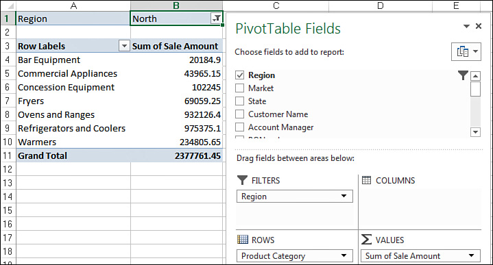
You might be asked to produce different reports for particular regions, markets, or products. Instead of building separate pivot table reports for every possible analysis scenario, you can use the Filter field to create a report filter. For example, you can create a region-filtered report by simply dragging the Region field to the Filters area and the Product Category field to the Rows area. This way, you can analyze one particular region at a time. Figure 2.15 shows the totals for just the North region.
Figure 2.15 With this setup, you not only can see revenues by product clearly, but also can click the Region drop-down to focus on one region.
Understanding the Recommended Pivot Table Feature
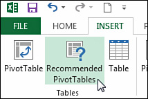
With Excel 2013, Microsoft introduced a feature called Recommended PivotTables. You can find this feature next to the PivotTable icon on the Insert tab (see Figure 2.16).
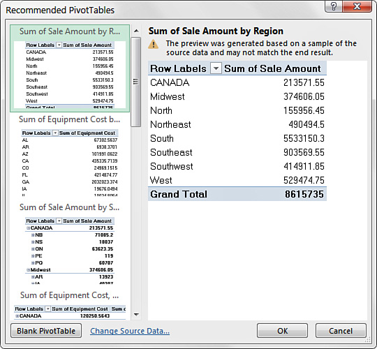
This feature is Microsoft’s way of getting you up and running with pivot tables by simply creating one for you. The idea is simple: Place your cursor in a tabular range of data and then click the Recommended PivotTables icon. Excel shows you a menu of pivot tables it thinks it can create for you, based on the data in your range (see Figure 2.17). When you find one that looks good to you, click it and then click OK to have Excel create it.
Figure 2.17 Choose from the menu of recommended pivot tables to have Excel automatically create a pivot table for you.
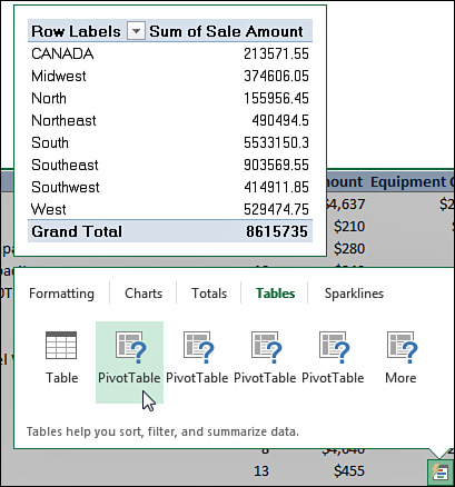
Another way to get to a recommended pivot table is to right-click anywhere in your data range and choose the Quick Analysis option. The context menu shown in Figure 2.18 activates, and you can select a recommended pivot table under the Tables section.
The reviews on this feature are mixed. On one hand, it does provide a quick and easy way to start a pivot table, especially for those of us who are not that experienced. On the other hand, Excel’s recommendations are rudimentary at best. You will often find that you need to rearrange, add, or manipulate fields in the created pivot table to suit your needs. Although Excel might get it right the first time, it’s unlikely that you will be able to leave the pivot table as is.
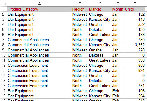
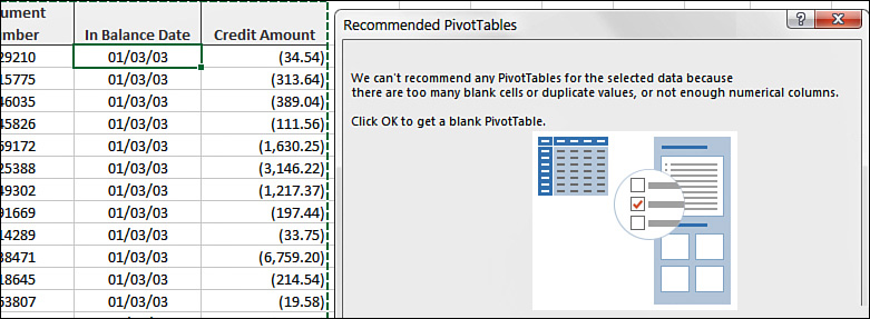
There is also a chance that Excel will simply not like the data range you pointed to. For example, the data in Figure 2.19 is a valid range, but Excel doesn’t like the repeating dates. So it pops up a message to indicate that there are too many duplicates to recommend a pivot table; however, it will gladly create a blank one.
Figure 2.19 When Excel can’t recommend a pivot table based on your data, it throws an error and gives you the option of starting with a blank pivot.
All in all, the Recommended PivotTables feature can be a nice shortcut for getting a rudimentary pivot table started, but it’s not a replacement for knowing how to create and manipulate pivot tables on your own.
Using Slicers
With Excel 2010, Microsoft introduced a feature called slicers. Slicers enable you to filter your pivot table in much the same way that the way Filter fields filter a pivot table. The difference is that slicers offer a user-friendly interface that enables you to easily see the current filter state.
Creating a Standard Slicer
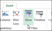
To understand the concept behind slicers, place your cursor anywhere inside your pivot table and then select the Insert tab on the ribbon. Click the Slicer icon (see Figure 2.20).
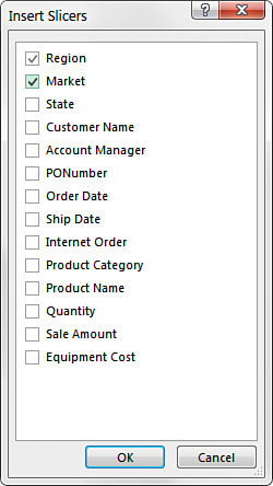
The Insert Slicers dialog, shown in Figure 2.21, opens. The idea is to select the dimensions you want to filter. In this example, the Region and Market slicers are selected.
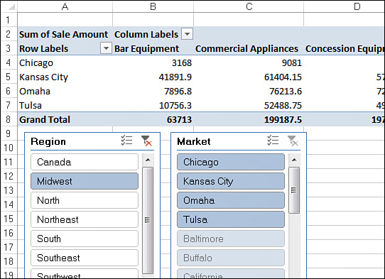
After the slicers are created, you can simply click the filter values to filter your pivot table. As you can see in Figure 2.22, clicking Midwest in the Region slicer filters your pivot table, and also the Market slicer responds by highlighting the markets that belong to the Midwest region.
Tip
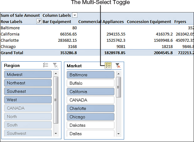
You can select multiple values by holding down the Ctrl key on your keyboard while selecting the needed filters. Alternatively, you can enable the Multi-Select toggle next to the filter icon at the top of the slicer.
In Figure 2.23, the Multi-Select toggle was enabled and then Baltimore, California, Charlotte, and Chicago were selected. Note that Excel highlights the selected markets in the Market slicer and also highlights their associated regions in the Region slicer.
Figure 2.23 The fact that they enable you to visually see the current filter state gives slicers a unique advantage over the Filter field.
Another advantage you gain with slicers is that you can tie each slicer to more than one pivot table. In other words, any filter you apply to your slicer can be applied to multiple pivot tables.
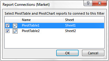
To connect a slicer to more than one pivot table, simply right-click the slicer and select Report Connections. The Report Connections dialog, shown in Figure 2.24, opens. Place a check next to any pivot table that you want to filter using the current slicer.
At this point, any filter applied via the slicer is applied to all the connected pivot tables. Again, slicers have a unique advantage over Filter fields in that they can control the filter state of multiple pivot tables. Filter fields can control only the pivot table in which they live.
It’s important to note that slicers are not part of a pivot table object. They are separate objects that you can use in a variety of ways. For a more detailed look at slicers, their functionality, and how to format them, pick up Que Publishing’s Special Edition Using Microsoft Excel 2016, by Bill Jelen.
Tip
Notice that in Figure 2.24, the list of pivot tables is a bit ambiguous (PivotTable1, PivotTable2). Excel automatically gives your pivot tables these generic names, which it uses to identify them. You can imagine how difficult it would be to know which pivot table is which when working with more than a handful of pivots. Therefore, you might want to consider giving your pivot tables user-friendly names so you can recognize them in dialog boxes such as the one you see in Figure 2.24.
You can easily change the name of a pivot table by placing your cursor anywhere inside the pivot table, selecting the Analyze tab, and entering a friendly name in the PivotTable Name input box found on the far left.
Creating a Timeline Slicer
The Timeline slicer (introduced with Excel 2013) works in the same way as a standard slicer in that it lets you filter a pivot table using a visual selection mechanism instead of the old Filter fields. The difference is that the Timeline slicer is designed to work exclusively with date fields, and it provides an excellent visual method to filter and group the dates in a pivot table.
Note
In order to create a Timeline slicer, your pivot table must contain a field where all the data is formatted as dates. This means that your source data table must contain at least one column where all the values are formatted as valid dates. If even only one value in the source date column is blank or not a valid date, Excel does not create a Timeline slicer.
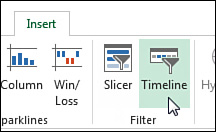
To create a Timeline slicer, place your cursor anywhere inside your pivot table, select the Insert tab on the ribbon, and then click the Timeline icon (see Figure 2.25).
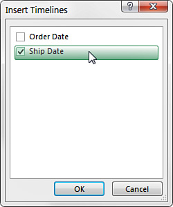
The Insert Timelines dialog shown in Figure 2.26 opens, showing you all the available date fields in the chosen pivot table. Here, you select the date fields for which you want to create slicers.
After your Timeline slicer is created, you can filter the data in your pivot table by using this dynamic data-selection mechanism. As you can see in Figure 2.27, clicking the April slicer filters the data in the pivot table to show only April data.
Figure 2.28 demonstrates how you can expand the slicer range with the mouse to include a wider range of dates in your filtered numbers.
Figure 2.28 You can expand the range on the Timeline slicer to include more data in the filtered numbers.
Want to quickly filter your pivot table by quarters? Well, you can easily do it with a Timeline slicer. Click the time period drop-down and select Quarters. As you can see in Figure 2.29, you also have the option of selecting Years or Days, if needed.
Be aware that Timeline slicers are not backward compatible, meaning that they are usable only in Excel 2013 and Excel 2016. If you open a workbook with Timeline slicers in Excel 2010 or earlier versions, the Timeline slicers are disabled.
Keeping Up with Changes in the Data Source
Let’s go back to the family portrait analogy. As years go by, your family will change in appearance and might even grow to include some new members. The family portrait that was taken years ago remains static and no longer represents the family today. So another portrait needs to be taken.
As time goes by, your data might change and grow with newly added rows and columns. However, the pivot cache that feeds your pivot table report is disconnected from your data source, so it cannot represent any of the changes you make to your date source until you take another snapshot.
The action of updating your pivot cache by taking another snapshot of your data source is called refreshing your data. There are two reasons you might have to refresh your pivot table report:
![]() Changes have been made to your existing data source.
Changes have been made to your existing data source.
![]() Your data source’s range has been expanded with the addition of rows or columns.
Your data source’s range has been expanded with the addition of rows or columns.
The following sections explain how to keep your pivot table synchronized with the changes in your data source.
Dealing with Changes Made to the Existing Data Source
If a few cells in your pivot table’s source data have changed due to edits or updates, you can refresh your pivot table report with a few clicks. Simply right-click inside your pivot table report and select Refresh. This selection takes another snapshot of your data set, overwriting your previous pivot cache with the latest data.
Note
You can also refresh the data in a pivot table by selecting Analyze from the PivotTable Tools tab in the ribbon and then choosing Refresh.
Tip
Clicking anywhere inside a pivot table activates the PivotTable Tools tab just above the main ribbon.
Dealing with an Expanded Data Source Range Due to the Addition of Rows or Columns
When changes have been made to your data source that affect its range (for example, if you’ve added rows or columns), you have to update the range being captured by the pivot cache.
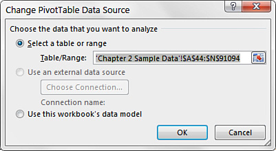
To do this, click anywhere inside the pivot table and then select Analyze from the PivotTable Tools tab in the ribbon. From here, select Change Data Source. This selection triggers the dialog shown in Figure 2.31.
Figure 2.31 The Change PivotTable Data Source dialog enables you to redefine the source data for your pivot table.
All you have to do here is update the range to include new rows and columns. After you have specified the appropriate range, click the OK button.
Sharing the Pivot Cache
You quite often need to analyze the same data set in multiple ways. In most cases, this process requires you to create separate pivot tables from the same data source. Keep in mind that every time you create a pivot table, you are storing a snapshot of the entire data set in a pivot cache. Every pivot cache that is created increases your memory usage and file size. For this reason, you should consider sharing your pivot cache.
Note
In situations where you need to create multiple pivot tables from the same data source, you can use the same pivot cache to feed multiple pivot tables. By using the same pivot cache for multiple pivot tables, you gain a certain level of efficiency when it comes to memory usage and file size.
In legacy versions of Excel, when you created a pivot table using a data set that was already being used in another pivot table, Excel actually gave you the option of using the same pivot cache. However, Excel 2016 does not give you such an option.
Instead, each time you create a new pivot table in Excel 2016, Excel automatically shares the pivot cache. Most of the time, this is beneficial: You can link as many pivot tables as you want to the same pivot cache with a negligible increase in memory and file size.
On the flip side, when you group one pivot table by month and year, all of the pivot tables are grouped in a similar fashion. If you want one pivot table by month and another pivot table by week, you have to force a separate pivot cache. You can force Excel to create a separate pivot cache by taking the following steps:
1. Press Alt+D+P on your keyboard to launch the Pivot Table Wizard.
2. Click the Next button to get past the first screen of the wizard.
3. On the second screen, select the range for your pivot table and click the Next button.
4. Excel displays a wordy message saying that you can use less memory if you click Yes. Instead, click No.
5. On the next screen, click the Finish button.
At this point, you have a blank pivot table that pulls from its own pivot cache.
If you already have an existing pivot table, you can use an alternative method for creating a separate pivot cache: Copy and paste the existing table to a new workbook and then copy and paste the pivot table back to a new sheet in the original workbook.
Saving Time with New Pivot Table Tools
Microsoft has invested a lot of time and effort in the overall pivot table experience. The results of these efforts are tools that make pivot table functionality more accessible and easier to use. The following sections look at a few of the tools that help you save time when managing pivot tables.
Deferring Layout Updates
The frustrating part of building a pivot table from a large data source is that each time you add a field to a pivot area, you are left waiting while Excel crunches through all that data. This can become a maddeningly time-consuming process if you have to add several fields to your pivot table.
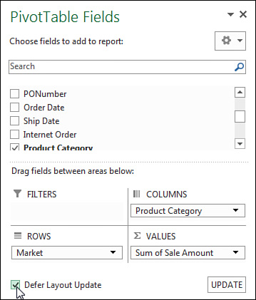
Excel 2016 offers some relief for this problem by providing a way to defer layout changes until you are ready to apply them. You can activate this option by clicking the relatively inconspicuous Defer Layout Update check box in the PivotTable Fields list, as shown in Figure 2.32.
Figure 2.32 Click the Defer Layout Update check box to prevent your pivot table from updating while you add fields.
Here’s how this feature works: With the Defer Layout Update check box selected, you prevent your pivot table from making real-time updates as you move your fields around without your pivot table. In Figure 2.32, notice that fields in the areas are not in the pivot table yet. The reason is that the Defer Layout Update check box is active. When you are ready to apply your changes, click the Update button on the lower-right corner of the PivotTable Fields list.
Note
Remember to remove the check from the Defer Layout Update check box when you are done building your pivot table. Leaving it checked results in your pivot table remaining in a state of manual updates, preventing you from using other features of the pivot table, such as sorting, filtering, and grouping.
Tip
Incidentally, the Defer Layout Update option is available through VBA. It can help improve the performance of any macro that automates the creation of pivot tables.
Note
For detailed information on how to use VBA to create pivot tables, refer to Chapter 13, “Using VBA to Create Pivot Tables.”
Starting Over with One Click
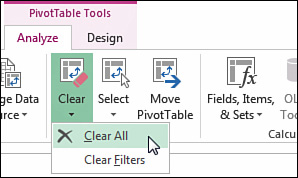
Often you might want to start from scratch when working with your pivot table layouts. Excel 2016 provides a simple way to essentially start over without deleting your pivot cache. Select Analyze under the PivotTable Tools tab and select the Clear drop-down. As you can see in Figure 2.33, this command enables you to either clear your entire pivot table layout or remove any existing filters you might have applied in your pivot table.
Figure 2.33 The Clear command enables you to clear your pivot table fields or remove the applied filters from your pivot table.
Relocating a Pivot Table
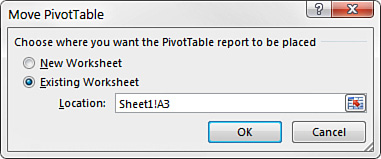
You might find that, after you have created a pivot table, you need to move it to another location. It might be in the way of other analyses on the worksheet, or you might simply need to move it to another worksheet. Although there are several ways to move a pivot table, the easiest is Excel 2016’s no-frills way: Select Analyze under the PivotTable Tools tab and select Move PivotTable. This icon activates the Move PivotTable dialog, shown in Figure 2.34. All you have to do here is specify where you want your pivot table moved.
Figure 2.34 The Move PivotTable dialog enables you to quickly move your pivot table to another location.
Next Steps
In Chapter 3, you’ll learn how to enhance your pivot table reports by customizing your fields, changing field names, changing summary calculations, applying formats to data fields, adding and removing subtotals, and using the Show As setting.

