Chapter 4
Managing Worksheets
In This Chapter
![]() Inserting and deleting columns and rows in a worksheet
Inserting and deleting columns and rows in a worksheet
![]() Splitting the worksheet into separate panes
Splitting the worksheet into separate panes
![]() Outlining data in a worksheet
Outlining data in a worksheet
![]() Inserting, deleting, and reordering worksheets in a workbook
Inserting, deleting, and reordering worksheets in a workbook
![]() Opening windows on different worksheets in a workbook
Opening windows on different worksheets in a workbook
![]() Working with multiple workbooks
Working with multiple workbooks
![]() Opening windows on different workbooks
Opening windows on different workbooks
![]() Consolidating worksheet data
Consolidating worksheet data
Being able to manage and reorganize the information in your spreadsheet is almost as important as being able to input data and edit it. As part of these skills, you need to know how to manipulate the columns and rows of a single worksheet, the various worksheets within a single workbook, and, at times, other workbooks that contain supporting or relevant data.
This chapter examines how to reorganize information in a single worksheet by inserting and deleting columns and rows, as well as how to apply outlining to data tables that enables you to expand and collapse details by showing and hiding columns and rows. It also covers how to reorganize and manipulate the actual worksheets in a workbook and discusses strategies for visually comparing and transferring data between the different workbooks that you have open for editing.
Reorganizing the Worksheet
Every Excel 2016 worksheet that you work with has 16,384 columns and 1,048,576 rows — no more, no less, regardless of how many or how few of its cells you use. As your spreadsheet grows, you may find it beneficial to rearrange the data so that it doesn’t creep. Many times, this involves deleting unnecessary columns and rows to bring the various data tables and lists in closer proximity to each other. At other times, you may need to insert new columns and rows in the worksheet so as to put a minimum of space between the groups of data.
Within the confines of this humongous worksheet space, your main challenge is often keeping tabs on all the information spread out throughout the sheet. At times, you may find that you need to split the worksheet window into panes so that you can view two disparate regions of the spreadsheet together in the same window and compare their data. For large data tables and lists, you may want to outline the worksheet data so that you can immediately collapse the information down to the summary or essential data and then just as quickly expand the information to show some or all of the supporting data.
Inserting and deleting columns and rows
The first thing to keep in mind when inserting or deleting columns and rows in a worksheet is that these operations affect all 1,048,576 rows in those columns and all 16,384 columns in those rows. As a result, you have to be sure that you’re not about to adversely affect data in unseen rows and columns of the sheet before you undertake these operations. Note that, in this regard, inserting columns or rows can be almost as detrimental as deleting them if, by inserting them, you split apart existing data tables or lists whose data should always remain together.
One way to guard against inadvertently deleting existing data or splitting apart a single range is to use the Zoom slider on the status bar to zoom out on the sheet and then check visually for intersecting groups of data in the hinterlands of the worksheet. You can do this quickly by dragging the Zoom slider button to the left to the 25% setting. Of course, even at the smallest zoom setting of 10%, you can see neither all the columns nor all the rows in the worksheet, and because everything’s so tiny at that setting, you can’t always tell whether or not the column or row you intend to fiddle with intersects those data ranges that you can identify.
Another way to check is to press End+→ or End+↓ to move the cell pointer from data range to data range across the column or row affected by your column or row deletion. Remember that pressing End plus an arrow key when the cell pointer is in a blank cell jumps the cell pointer to the next occupied cell in its row or column. That means if you press End+→ when the cell pointer is in row 52 and the pointer jumps to cell XFD52 (the end of the worksheet in that row), you know that there isn’t any data in that row that would be eliminated by your deleting that row or shifted up or down by your inserting a new row. So too, if you press End+↓ when the cell pointer is in column D and the cell pointer jumps down to cell D1048576, you’re assured that no data is about to be purged or shifted left or right by that column’s deletion or a new column’s insertion at that point.
When you’re sure that you aren’t about to make any problems for yourself in other, unseen parts of the worksheet by deleting or inserting columns, you’re ready to make these structural changes to the worksheet.
Eradicating columns and rows
To delete columns or rows of the worksheet, select them by clicking their column letters or row numbers in the column or row header and then click the Delete button in the Cells group on the Ribbon’s Home tab. Remember that you can select groups of columns and rows by dragging through their letters and numbers in the column or row header. You can also select nonadjacent columns and rows by holding down the Ctrl key as you click them.
When you delete a column, all the data entries within the cells of that column are immediately zapped. At the same time, all remaining data entries in succeeding columns to the right move left to fill the blank left by the now-missing column. When you delete a row, all the data entries within the cells of that row are immediately eliminated, and the remaining data entries in rows below move up to fill in the gap left by the missing row.
 You can also delete rows and columns of the worksheet corresponding to those that are a part of the current cell selection in the worksheet by clicking the drop-down button attached to the Delete command button on the Home tab of the Ribbon and then choosing the Delete Sheet Rows or Delete Sheet Columns option, respectively, from its drop-down menu. If you find you can’t safely delete an entire column or row, delete the cells you need to get rid of in the particular region of the worksheet instead by selecting them and then choosing the Delete Cells option from the Delete button’s drop-down menu. (See Book II, Chapter 3 for details.)
 Remember that pressing the Delete key is not the same as clicking the Delete button on the Home tab of the Ribbon. When you press the Delete key after selecting columns or rows in the worksheet, Excel simply clears the data entries in their cells without adjusting any of the existing data entries in neighboring columns and rows. Click the Delete command button on the Home tab when your purpose is both to delete the data in the selected columns or rows and to fill in the gap by adjusting the position of entries to the right and below the ones you eliminate.
 Should your row or column deletions remove data entries referenced in formulas, the #REF! error value replaces the calculated values in the cells of the formulas affected by the elimination of the original cell references. You must then either restore the deleted rows or columns or re-create the original formula and then recopy it to get rid of these nasty formula errors. (See Book III, Chapter 2 for more on error values in formulas.)
Adding new columns and rows
To insert a new column or row into the worksheet, you select the column or row where you want the new blank column or row to appear (again by clicking its column letter or row number in the column or row header) and then click the Insert command button in the Cells group of the Ribbon’s Home tab or right-click and select Insert on the pop-up menu.
When you insert a blank column, Excel moves the existing data in the selected column to the column to the immediate right, while simultaneously moving any other columns of data on the right over one. When you insert the blank row, Excel moves the existing data in the selected row down to the row immediately underneath, while simultaneously adjusting any other rows of existing data that fall below it down by one.
To insert multiple columns or rows at one time in the worksheet, select the columns or rows where you want the new blank columns or rows to appear (by dragging through their column letters and row numbers in the column and row header) before you click the Insert command button on the Home tab of the Ribbon.
You can also insert new rows and columns of the worksheet corresponding to those that are a part of the current cell selection in the worksheet by clicking the drop-down button attached to the Insert command button on the Home tab and then choosing the Insert Sheet Rows or Insert Sheet Columns option, respectively, from its drop-down menu. If you find that you can’t safely insert an entire column or row, insert the blank cells you need in the particular region of the worksheet instead by selecting their cells and then choosing the Insert Cells option from the Insert command button’s drop-down menu. (See Book II, Chapter 3 for details.)
Whenever your column or row insertions reposition data entries that are referenced in other formulas in the worksheet, Excel automatically adjusts the cell references in the formulas affected to reflect the movement of their columns left or right, or rows up or down.
Splitting the worksheet into panes
Excel enables you to split the active worksheet window into two or four panes. After splitting up the window into panes, you can use the Excel workbook’s horizontal and vertical scroll bars to bring different parts of the same worksheet into view. This is great for comparing the data in different sections of a table that would otherwise not be legible if you zoomed out far enough to have both sections displayed in the worksheet window.
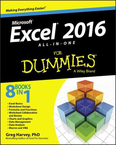
To split the worksheet window into two horizontal panes, position the cell pointer in column A of the worksheet in the cell whose top border marks the place where you want the horizontal division to take place before clicking the Split button on the View tab of the Ribbon (or pressing Alt+WS). Excel then splits the window into two horizontal panes with the cell pointer in the upper-left corner of the lower pane. (See Figure 4-1.)
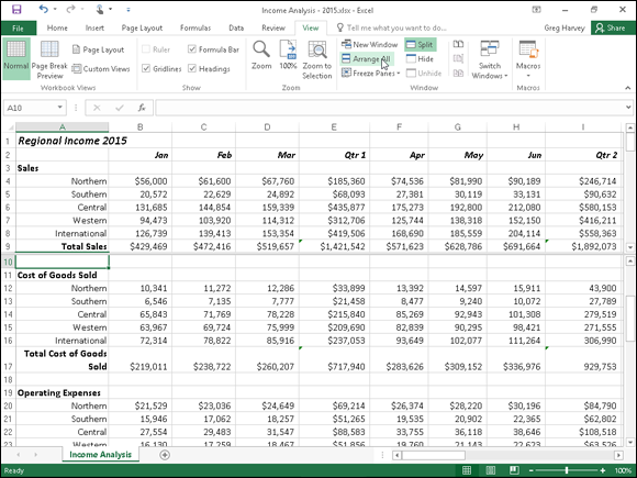
Figure 4-1: The Regional Income worksheet with the window divided into two horizontal panes at row 10.
To split the window into two vertical panes, you put the cell pointer in the first row of the column where the split is to occur. To split the window into four panes, you place the cell pointer in the cell in the column to the right of the vertical dividing line and the row below the horizontal dividing line so that the cell pointer will be in the upper-left corner of the lower-right pane when the split occurs (as shown in Figure 4-3).
Excel displays the borders of the window panes you create in the document window with a bar that ends with the vertical or horizontal split bar. To modify the size of a pane, you position the white-cross pointer on the appropriate dividing bar. Then as soon as the pointer changes to a double-headed arrow, drag the bar until the pane is the correct size and release the mouse button.
When you split a window into panes, Excel automatically synchronizes the scrolling, depending on how you split the worksheet. When you split a window into two horizontal panes, as shown in Figure 4-1, the worksheet window contains a single horizontal scroll bar and two separate vertical scroll bars. This means that all horizontal scrolling of the two panes is synchronized, while the vertical scrolling of each pane remains independent.
When you split a window into two vertical panes, as shown in Figure 4-2, the situation is reversed. The worksheet window contains a single vertical scroll bar and two separate horizontal scroll bars. This means that all vertical scrolling of the two panes is synchronized, while horizontal scrolling of each pane remains independent.
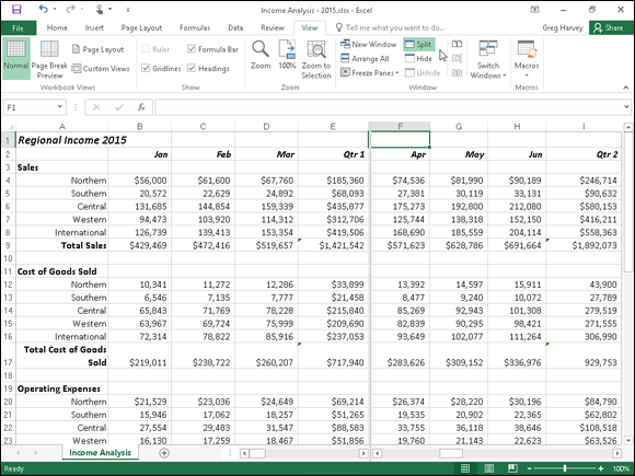
Figure 4-2: The Regional Income worksheet with the window divided into two vertical panes at column F.
When you split a window into two horizontal and two vertical panes, as shown in Figure 4-3, the worksheet window contains two horizontal scroll bars and two separate vertical scroll bars. This means that vertical scrolling is synchronized in the top two window panes when you use the top vertical scroll bar and synchronized for the bottom two window panes when you use the bottom vertical scroll bar. Likewise, horizontal scrolling is synchronized for the left two window panes when you use the horizontal scroll bar on the left, and it’s synchronized for the right two window panes when you use the horizontal scroll bar on the right.

Figure 4-3: Splitting the worksheet window into four panes: two horizontal and two vertical at cell F10.
To remove all panes from a window when you no longer need them, you simply click the Split button on the View tab of the Ribbon, press Alt+WS, or drag the dividing bar (with the black double-headed split arrow cursor) either for the horizontal or vertical pane until you reach one of the edges of the worksheet window. You can also remove a pane by positioning the mouse pointer on a pane-dividing bar and then, when it changes to a double-headed split arrow, double-clicking it.
 Remember that on a touchscreen, you can also remove the panes in a worksheet by directly double-tapping the pane-dividing bar with your finger or stylus.
Keep in mind that you can freeze panes in the window so that information in the upper pane and/or in the leftmost pane remains in the worksheet window at all times, no matter what other columns and rows you scroll to or how much you zoom in and out on the data. (See Book II, Chapter 3 for more on freezing panes.)
Outlining worksheets
The Outline feature enables you to control the level of detail displayed in a data table or list in a worksheet. To be able to outline a table or list, the data must use a uniform layout with a row of column headings identifying each column of data and summary rows that subtotal and total the data in rows above (like the CG Media Sales table shown in Figure 4-4).
Figure 4-4: Automatic outline applied to the CG Music sales table with three levels of detail displayed.
After outlining a table or list, you can condense the table’s display when you want to use only certain levels of summary information, and you can just as easily expand the outlined table or list to display various levels of detail data as needed. Being able to control which outline level is displayed in the worksheet makes it easy to print summary reports with various levels of data (see Book II, Chapter 5) as well as to chart just the summary data (see Book V, Chapter 1).
Spreadsheet outlines are a little different from the outlines you created in high school and college. In those outlines, you placed the headings at the highest level (I.) at the top of the outline with the intermediate headings indented below. Most worksheet outlines, however, seem backward in the sense that the highest level summary row and column are located at the bottom and far right of the table or list of data, with the columns and rows of intermediate supporting data located above and to the left of the summary row and column.
The reason that worksheet outlines often seem “backward” when compared to word-processing outlines is that, most often, to calculate your summary totals in the worksheet, you naturally place the detail levels of data above the summary rows and to the left of the summary columns that total them. When creating a word-processing outline, however, you place the major headings above subordinate headings, while at the same time indenting each subordinate level, reflecting the way we read words from left to right and down the page.
Outlines for data tables (as opposed to data lists) are also different from regular word-processing outlines because they outline the data in not one, but two hierarchies: a vertical hierarchy that summarizes the row data, and a horizontal hierarchy that summarizes the column data. (You don’t get much of that in your regular term paper!)
Creating the outline
To create an outline from a table of data, position the cell pointer in the table or list containing the data to be outlined and then click the Auto Outline option on the Group command button’s drop-down menu on the Data tab on the Ribbon (or press Alt+AGA).
By default, Excel assumes that summary rows in the selected data table are below their detail data, and summary columns are to the right of their detail data, which is normally the case. If, however, the summary rows are above the detail data, and summary columns are to the left of the detail data, Excel can still build the outline.
Simply start by clicking the Dialog Box launcher in the lower-right corner of the Outline group on the Data tab of the Ribbon to open the Settings dialog box. In the Settings dialog box, clear the check marks from the Summary Rows below Detail and/or Summary Columns to Right of Detail check boxes in the Direction section. Also, you can have Excel automatically apply styles to different levels of the outline by selecting the Automatic Styles check box. (For more information on these styles, see the “Applying outline styles” section, later in this chapter.) To have Excel create the outline, click the Create button — if you click the OK button, the program simply closes the dialog box without outlining the selected worksheet data.
Figure 4-4 shows you the first part of the outline created by Excel for the CG Music 2015 Sales worksheet. Note the various outline symbols that Excel added to the worksheet when it created the outline. Figure 4-4 identifies most of these outline symbols (the Show Detail button with the plus sign is not displayed in this figure), and Table 4-1 explains their functions.
Table 4-1 Outline Buttons
Button |
Function |
Row Level (1-8) and Column Level (1-8) |
Displays a desired level of detail throughout the outline (1, 2, 3, and so on up to 8). When you click an outline’s level bar rather than a numbered Row Level or Column Level button, Excel hides only that level in the worksheet display, the same as clicking the Hide Detail button (explained below). |
Show Detail (+) |
Expands the display to show the detail rows or columns that have been collapsed. |
Hide Detail (–) |
Condenses the display to hide the detail rows or columns that are included in its row or column level bar. |
If you don’t see any of the outline doodads identified in Figure 4-4 and Table 4-1, this means that the Show Outline Symbols If an Outline Is Applied check box in the Displays Options for This Worksheet section of the Advanced tab in the Excel Options dialog box (Alt+FTA) is not checked. All you have to do is press Ctrl+8 to display the outline symbols. Keep in mind that Ctrl+8 is a toggle that you can press again to hide the outline symbols.
You can have only one outline per worksheet. If you’ve already outlined one table and then try to outline another table on the same worksheet, Excel will display the Modify Existing Outline alert box when you choose the Outline command. If you click OK, Excel adds the outlining for the new table to the existing outline for the first table (even though the tables are nonadjacent). To create separate outlines for different data tables, you need to place each table on a different worksheet of the workbook.
Applying outline styles
You can apply predefined row and column outline styles to the table or list data. To apply these styles when creating the outline, be sure to select the Automatic Styles check box in the Settings dialog box before you click its Create button, opened by clicking the Dialog Box launcher in the Outline group on the Data tab of the Ribbon. If you didn’t select this check box in the Settings dialog box before you created the outline, you can do so afterwards by selecting all the cells in the outlined table of data, opening the Settings dialog box, clicking the Automatic Styles check box to put a check mark in it, and then clicking the Apply Styles button before you click OK.
Figure 4-5 shows you the sample CG Music Sales table after I applied the automatic row and column styles to the outlined table data. In this example, Excel applied two row styles (RowLevel_1 and RowLevel_2) and two column styles (ColLevel_1 and ColLevel_2) to the worksheet table.
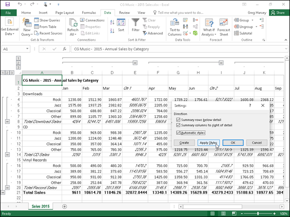
Figure 4-5: Worksheet outline after applying automatic styles with the Settings dialog box.
The RowLevel_1 style is applied to the entries in the first-level summary row (row 21) and makes the font appear in bold. The ColLevel_1 style is applied to the data in the first-level summary column (column R, which isn’t shown in the figure), and it, too, simply makes the font bold. The RowLevel_2 style is applied to the data in the second-level rows (rows 8 and 20), and this style adds italics to the font. The ColLevel_2 style is applied to all second-level summary columns (columns E, I, M, and Q), and it also italicizes the font. (Note that columns M and Q are also not visible in Figure 4-5.)
Sometimes Excel can get a little finicky about applying styles to an existing outline. If, in the Settings dialog box, you select the Automatic Styles check box, click the Apply Styles button, and nothing happens to your outline, simply click the OK button to close the Settings dialog box. Then, re-create the outline by selecting the Auto Outline option on the Group drop-down list on the Data tab. Excel displays an alert dialog box asking you to confirm that you want to modify the existing outline. As soon as you click OK, Excel redisplays your outline, this time with the automatic styles applied.
Displaying and hiding different outline levels
The real effectiveness of outlining worksheet data becomes apparent as soon as you start using the various outline symbols to change the way the table data are displayed in the worksheet. By clicking the appropriate row or column level symbol, you can immediately hide detail rows and columns to display just the summary information in the table. For example, Figure 4-6 shows you the CG Music Sales table after clicking the number 2 Row Level button and number 2 Column Level button. Here, you see only the first- and second-level summary information, that is, the totals for the quarterly and annual totals for the three types of music sales.

Figure 4-6: Collapsed worksheet outline showing first- and secondary-level summary information.
You can also hide and display levels of the outlined data by positioning the cell cursor in the column or row and then clicking the Hide Detail (the one with the red minus sign) or the Show Detail button (the one with the green minus sign) in the Outline group of the Data tab of the Ribbon. Or you can press the hot keys, Alt+AH, to hide an outline level, and Alt+AJ to redisplay the level. The great thing about using these command buttons or their hot key equivalents is that they work even when the outline symbols are not displayed in the worksheet.
Figure 4-7 shows you the same table, this time after clicking the number 1 Row Level button and number 1 Column Level button. Here, you see only the first-level summary for the column and the row, that is, the grand total of the annual CG Music sales. To expand this view horizontally to see the total sales for each quarter, you would simply click the number 2 Column Level button. To expand this view even further horizontally to display each monthly total in the worksheet, you would click the number 3 Column Level button. So too, to expand the outline vertically to see totals for each type of media, you would click the number 2 Row Level button. To expand the outline one more level vertically so that you can see the sales for each type of music as well as each type of media, you would click the number 3 Row Level button.

Figure 4-7: Totally collapsed worksheet outline showing only the first-level summary information.
When displaying different levels of detail in a worksheet outline, you can use the Hide Detail and Show Detail buttons along with the Row Level and Column Level buttons. For example, Figure 4-8 shows you another view of the CG Music outlined sales table. Here, in the horizontal dimension, you see all three column levels have been expanded, including the monthly detail columns for each quarter. In the vertical dimension, however, only the detail rows for the Download sales have been expanded. The detail rows for the CD and Vinyl Record sales are still collapsed.
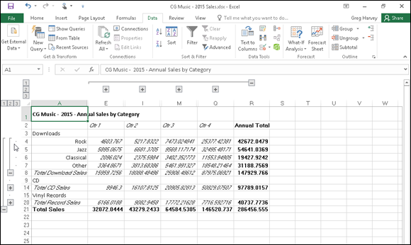
Figure 4-8: Worksheet outline expanded to show only details for Download sales for all four quarters.
To create this view of the outline, you simply click the number 2 Column Level and Row Level buttons, and then click only the Show Detail (+) button located to the left of the Total Download Sales row heading. When you want to view only the summary-level rows for each media type, you can click the Hide Detail (–) button to the left of the Total Download Sales heading, or you can click its level bar (drawn from the collapse symbol up to the first music type to indicate all the detail rows included in that level).
Excel adjusts the outline levels displayed on the screen by hiding and redisplaying entire columns and rows in the worksheet. Therefore, keep in mind that changes that you make that reduce the number of levels displayed in the outlined table also hide the display of all data outside of the outlined table that are in the affected rows and columns.
After selecting the rows and columns you want displayed, you can then remove the outline symbols from the worksheet display to maximize the amount of data displayed onscreen. To do this, simply press Ctrl+8.
Manually adjusting the outline levels
Most of the time, Excel’s Auto Outline feature correctly outlines the data in your table. Every once in a while, however, you will have to manually adjust one or more of the outline levels so that the outline’s summary rows and columns include the right detail rows and columns. To adjust levels of a worksheet outline, you must select the rows or columns that you want to promote to a higher level (that is, one with a lower level number) in the outline and then click the Group button on the far right side of the Data tab of the Ribbon. If you want to demote selected rows or columns to a lower level in the outline, select the rows or columns with a higher level number and then click the Ungroup button on the Data tab.
Before you use the Group and Ungroup buttons to change an outline level, you must select the rows or columns that you want to promote or demote. To select a particular outline level and all the rows and columns included in that level, you need to display the outline symbols (Ctrl+8), and then hold down the Shift key as you click its collapse or expand symbol. Note that when you click an expand symbol, Excel selects not only the rows or columns visible at that level, but all the hidden rows and columns included in that level as well. If you want to select only a particular detail or summary row or column in the outline, you can click that row number or column letter in the worksheet window, or you can hold down the Shift key and click the dot (period) to the left of the row number or above the column letter in the outline symbols area.
If you select only a range of cells in the rows or columns (as opposed to entire rows and columns) before you click the Group and Ungroup command buttons, Excel displays the Group or Ungroup dialog box, which contains a Rows and Columns option button (with the Rows button selected by default). To promote or demote columns instead of rows, click the Columns option button before you select OK. To close the dialog box without promoting or demoting any part of the outline, click Cancel.
To see how you can use the Group and Ungroup command buttons on the Data tab of the Ribbon to adjust outline levels, consider once again the CG Music Sales table outline. When Excel created this outline, the program did not include row 3 (which contains only the row heading, Downloads) in the outline. As a result, when you collapse the rows by selecting the number 1 Row Level button to display only the first-level Total Sales summary row (refer to Figure 4-7), this Download row heading remains visible in the table, even though it should have been included and thereby hidden along with the other summary and detail rows.
You can use the Group command button to move this row (3) down a level so that it is included in the first level of the outline. You simply click the row number 3 to select the row and then click the Group command button on the Data tab (or press Alt+AGG). Figure 4-9 shows you the result of doing this. Notice how the outside level bar (for level 1) now includes this row. Now, when you collapse the outline by clicking the number 1 row level button, the heading in row 3 is hidden as well. (See Figure 4-10.)
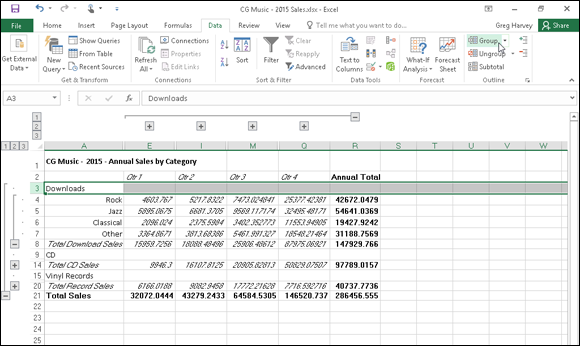
Figure 4-9: Manually adjusting the level 1 rows in the worksheet outline.

Figure 4-10: Collapsing the adjusted worksheet outline to the first level summary information.
Removing an outline
To delete an outline from your worksheet, you click the drop-down button attached to the Ungroup button on the Data tab of the Ribbon and then choose the Clear Outline option from its drop-down menu (or you press Alt+AUC). Note that removing the outline does not affect the data in any way — Excel merely removes the outline structure. Also note that it doesn’t matter what state the outline is in at the time you select this command. If the outline is partially or totally collapsed, deleting the outline automatically displays all the hidden rows and columns in the data table or list.
Keep in mind that restoring an outline that you’ve deleted is not one of the commands that you can undo (Ctrl+Z). If you delete an outline by mistake, you must re-create it all over again. For this reason, most often you’ll want to expand all the outline levels (by clicking the lowest number column and row level button) and then hide all the outline symbols by pressing Ctrl+8 rather than permanently remove the outline. Note that if you press Ctrl+8 when your spreadsheet table isn’t yet outlined, Excel displays an alert dialog box indicating that it can’t show the outline symbols because no outline exists. This alert also asks you whether you want to create an outline. To go ahead and outline the spreadsheet, click OK or press Enter. To remove the alert dialog box without creating an outline, click Cancel.
Creating different custom views of the outline
After you’ve created an outline for your worksheet table, you can create custom views that display the table in various levels of detail. Then, instead of having to display the outline symbols and manually click the Show Detail and Hide Detail buttons or the appropriate row level buttons and/or column level buttons to view a particular level of detail, you simply select the appropriate outline view in the Custom Views dialog box (View ⇒ Custom Views or Alt+WCV).
When creating custom views of outlined worksheet data, be sure that you leave the Hidden Rows, Columns, and Filter Settings check box selected in the Include in View section of the Add View dialog box. (See Book II, Chapter 3 for details on creating and using custom views in a worksheet.)
Reorganizing the Workbook
Any new workbook that you open already comes with a single blank worksheet. Although most of the spreadsheets you create and work with may never wander beyond the confines of this one worksheet, you do need to know how to organize your spreadsheet information three-dimensionally for those rare occasions when spreading all the information out in one humongous worksheet is not practical. However, the normal, everyday problems related to keeping on top of the information in a single worksheet can easily go off the scale when you begin to use multiple worksheets in a workbook. For this reason, you need to be sure that you are fully versed in the basics of using more than one worksheet in a workbook.
To move between the sheets in a workbook, you can click the sheet tab for that worksheet or press Ctrl+PgDn (next sheet) or Ctrl+PgUp (preceding sheet) until the sheet is selected. If the sheet tab for the worksheet you want is not displayed on the scroll bar at the bottom of the document window, use the tab scrolling buttons (the buttons with the left- and right-pointing triangles) to bring it into view.
To use the tab scrolling buttons, click the one with the right-pointing triangle to bring the next sheet into view and click the one with the left-pointing triangle to bring the preceding sheet into view. Ctrl-click the tab scrolling buttons with the directional triangles to display the very first or very last group of sheet tabs in a workbook. Ctrl-clicking the button with the triangle pointing left to a vertical line brings the first group of sheet tabs into view; Ctrl-clicking the button with the triangle pointing right to a vertical line brings the last group of sheet tabs into view. When you scroll sheet tabs to find the one you’re looking for, for heaven’s sake, don’t forget to click the desired sheet tab to make the worksheet current.
Excel 2016 indicates that there are more worksheets in a workbook whose tabs are not visible by adding a continuation button (indicated by an ellipsis, that is, three dots in row) either immediately following the last visible tab on the right or the first visible tab on the left. Keep in mind that you can also scroll the next or previously hidden sheet tab into view by clicking the continuation button on the right of the last visible sheet tab or left of the first visible tab, respectively.
Renaming sheets
The sheet tabs shown at the bottom of each workbook are the keys to keeping your place in a workbook. To tell which sheet is current, you have only to look at which sheet tab appears on the top, matches the background of the other cells in the worksheet, and has its name displayed in bold type and underlined.
When you add new worksheets to a new workbook, the sheet tabs are all the same width because they all have the default sheet names (Sheet1, Sheet2, and so on). As you assign your own names to the sheets, the tabs appear either longer or shorter, depending on the length of the sheet tab name. Just keep in mind that the longer the sheet tabs, the fewer you can see at one time, and the more sheet tab scrolling you’ll have to do to find the worksheet you want.
To rename a worksheet, you take these steps:
Press Ctrl+PgDn until the sheet you want to rename is active, or click its sheet tab if it’s displayed at the bottom of the workbook window.
Don’t forget that you have to select and activate the sheet you want to rename, or you end up renaming whatever sheet happens to be current at the time you perform the next step.
Choose Rename Sheet from the Format button’s drop-down menu on the Home tab, press Alt+HOR, or right-click the sheet tab and then choose Rename from its shortcut menu.
When you choose this command, Excel selects the current name of the tab and positions the insertion point at the end of the name.
- Replace or edit the name on the sheet tab and then press the Enter key.
When you rename a worksheet in this manner, keep in mind that Excel then uses that sheet name in any formulas that refer to cells in that worksheet. So, for instance, if you rename Sheet2 to 2016 Sales and then create a formula in cell A10 of Sheet1 that adds its cell B10 to cell C34 in Sheet2, the formula in cell A10 becomes:
=B10+'2016 Sales'!C34
This is in place of the more obscure =B10+Sheet2!C34. For this reason, keep your sheet names short and to the point so that you can easily and quickly identify the sheet and its data without creating excessively long formula references.
Right-click either of the two tab scrolling buttons to display the Activate dialog box. This dialog box displays the names of all the worksheets in the current workbook in their current order. You can then scroll to and activate any of the sheets simply by selecting them followed by OK or by double-clicking them.
Designer sheets
Excel 2016 makes it easy to color-code the worksheets in your workbook. This makes it possible to create a color scheme that helps either identify or prioritize the sheets and the information they contain (as you might with different colored folder tabs in a filing cabinet).
When you color a sheet tab, note that the tab appears in that color only when it’s not the active sheet. The moment you select a color-coded sheet tab, it becomes white with just a bar of the assigned color appearing under the sheet name. Note, too, that when you assign darker colors to a sheet tab, Excel automatically reverses out the sheet name text to white when the worksheet is not active.
Color coding sheet tabs
To assign a new color to a sheet tab, follow these three steps:
Press Ctrl+PgDn until the sheet whose tab you want to color is active, or click its sheet tab if it’s displayed at the bottom of the workbook window.
Don’t forget that you have to select and activate the sheet whose tab you want to color, or you end up coloring the tab of whatever sheet happens to be current at the time you perform the next step.
- Click the Format button on the Home tab and then highlight Tab Color, press Alt+HOT, or right-click the tab and then highlight Tab Color on the shortcut menu to display its pop-up color palette.
- Click the color swatch in the color palette with the color and shade you want to assign to the current sheet tab.
To remove color-coding from a sheet tab, click the No Color option at the bottom of the pop-up color palette (Alt+HOT) after selecting it to make the worksheet active.
Assigning a graphic image as the sheet background
If coloring the sheet tabs isn’t enough for you, you can also assign a graphic image to be used as the background for all the cells in the entire worksheet. Just be aware that the background image must either be very light in color or use a greatly reduced opacity in order for your worksheet data to be read over the image. This probably makes most graphics that you have readily available unusable as worksheet background images. It can, however, be quite effective if you have a special corporate watermark graphic (as with the company’s logo at extremely low opacity) that adds just a hint of a background without obscuring the data being presented in its cells.
To add a local graphic file as the background for your worksheet, take these steps:
Press Ctrl+PgDn until the sheet to which you want to assign the graphic as the background is active, or click its sheet tab if it’s displayed at the bottom of the workbook window.
Don’t forget that you have to select and activate the sheet to which the graphic file will act as the background, or you end up assigning the file to whatever sheet happens to be current at the time you perform the following steps.
Click the Background command button in the Page Setup group of the Page Layout tab or press Alt+PG.
Doing this opens the Insert Pictures dialog box, where you select the graphics file whose image is to become the worksheet background.
Click the Browse button to the right of the From a File link.
Excel opens the Sheet Background dialog box, where you select the file containing the graphic image you want to use.
- Open the folder that contains the image you want to use and then click its graphic file icon before you click the Insert button.
As soon as you click the Insert button, Excel closes the Sheet Background dialog box, and the image in the selected file becomes the background image for all cells in the current worksheet. (Usually, the program does this by stretching the graphic so that it takes up all the cells that are visible in the Workbook window. In the case of some smaller images, the program does this by tiling the image so that it’s duplicated across and down the viewing area.)
Keep in mind that a graphic image that you assign as the worksheet background doesn’t appear in the printout, unlike the pattern and background colors that you assign to ranges of cells in the sheet.
To remove a background image, you simply click the Delete Background command button on the Page Layout tab of the Ribbon (which replaces the Background button the moment you assign a background image to a worksheet) or press Alt+PSB again, and Excel immediately clears the image from the entire worksheet.
You can also turn online graphics into worksheet backgrounds. Simply select the Bing Image Search text box (to insert a web graphic). Then, perform a search for the image you want to use. (See Book V, Chapter 2 for details.) When you locate the online graphic you want to use, double-click its thumbnail to download the image and insert it into the current worksheet as the sheet’s background.
Adding and deleting sheets
You can add as many worksheets to the single Sheet1 that comes as part of every new workbook as you need in building your spreadsheet model. To add a new worksheet, click the New Sheet button, which always appears on its own tab immediately after the last sheet tab in the workbook (with the plus inside a circle icon).
Excel then inserts a new sheet at the back of the default Sheet1 worksheet in the workbook (and immediately in front of the tab with the New Sheet button), and the program assigns it the next available sheet number (as in Sheet2, Sheet3, Sheet4, and so on).
You can also insert a new sheet (and not necessarily a blank worksheet) into the workbook by right-clicking a sheet tab and then clicking Insert at the top of the tab’s shortcut menu. Excel opens the Insert dialog box containing different file icons that you can select — Chart, MS Excel 4.0 Macro, and MS Excel 5.0 Dialog, along with a variety of different worksheet templates — to insert a specialized chart sheet (see Book V, Chapter 1), macro sheet (Book VIII, Chapter 1), or worksheet following a template design (Book II, Chapter 1). Note that when you insert a new sheet using the Insert dialog box, Excel inserts the new sheet in front of the worksheet that’s active (and not at the end of the workbook as when you insert a worksheet by clicking the New Sheet button).
If you find that a single worksheet just never seems sufficient for the kind of spreadsheets you normally create, you can change the default number of sheets that are automatically available in all new workbook files that you open. To do this, open the General tab of the Excel Options dialog box (File ⇒ Options or Alt+FT), and then enter a number in the Include This Many Sheets text box or select the number with the spinner buttons (from 2 up to a maximum of 255). You can’t go lower than 1 because a workbook with no worksheet is no workbook at all.
To remove a worksheet, make the sheet active and then click the drop-down button attached to the Delete button on the Home tab of the Ribbon and choose Delete Sheet from its drop-down menu — you can also press Alt+HDS or right-click its tab and then choose Delete from its shortcut menu. If Excel detects that the worksheet contains some data, the program then displays an alert dialog box cautioning you that data may exist in the worksheet you’re just about to zap. To go ahead and delete the sheet (data and all), you click the Delete button. To preserve the worksheet, click Cancel or press the Escape key.
Deleting a sheet is one of those actions that you can’t undo with the Undo button on the Quick Access toolbar. This means that after you click the Delete button, you’ve kissed your worksheet goodbye, so please don’t do this unless you’re certain that you aren’t dumping needed data. Also, keep in mind that you can’t delete a worksheet if that sheet is the only one in the workbook until you’ve inserted another blank worksheet: Excel won’t allow a workbook file to be completely sheetless.
Changing the sheets
Excel makes it easy to rearrange the order of the sheets in your workbook. To move a sheet, click its sheet tab and drag it to the new position in the row of tabs. As you drag, the pointer changes shape to an arrowhead on a dog-eared piece of paper, and you see a black triangle pointing downward above the sheet tabs. When this triangle is positioned over the tab of the sheet that is to follow the one you’re moving, release the mouse button.
If you need to copy a worksheet to another position in the workbook, hold down the Ctrl key as you click and drag the sheet tab. When you release the mouse button, Excel creates a copy with a new sheet tab name based on the number of the copy and the original sheet name. For example, if you copy Sheet1 to a new place in the workbook, the copy is renamed Sheet1 (2). You can then rename the worksheet whatever you want.
You can also rearrange the sheets in your workbook using the Move or Copy dialog box opened by right-clicking a sheet tab and then choosing the Move or Copy command from the shortcut menu. Then, click the name of the worksheet that you want the currently active worksheet to now precede in the Before Sheet list box and selecting OK.
Group editing
One of the nice things about a workbook is that it enables you to edit more than one worksheet at a time. Of course, you should be concerned with group editing only when you’re working on a bunch of worksheets that share essentially the same layout and require the same type of formatting.
For example, suppose that you have a workbook that contains annual sales worksheets (named YTD10, YTD11, and YTD12) for three consecutive years. The worksheets share the same layout (with months across the columns and quarterly and annual totals, locations, and types of sales down the rows) but lack standard formatting.
To format any part of these three worksheets in a single operation, you simply resort to group editing, which requires selecting the three sales worksheets. Simply click the YTD10, YTD11, and YTD12 sheet tabs as you hold down the Ctrl key, or you can click the YTD10 tab and then hold down the Shift key as you click the YTD12 tab.
After you select the last sheet, the message [Group] appears in the title bar of the active document window (with the YTD10 worksheet, in this case).
The [Group] indicator lets you know that any editing change you make to the current worksheet will affect all the sheets that are currently selected. For example, if you select a row of column headings and add bold and italics to the headings in the current worksheet, the same formatting is applied to the same cell selection in all three sales sheets. All headings in the same cell range in the other worksheets are now in bold and italics. Keep in mind that you can apply not only formatting changes to a cell range, but also editing changes, such as replacing a cell entry, deleting a cell’s contents, or moving a cell selection to a new place in the worksheet. These changes also affect all the worksheets you have selected as long as they’re grouped together.
After you are finished making editing changes that affect all the grouped worksheets, you can break up the group by right-clicking one of the sheet tabs and then choosing Ungroup Sheets at the top of the shortcut menu. As soon as you break up the group, the [Group] indicator disappears from the title bar, and thereafter, any editing changes that you make affect only the cells in the active worksheet.
To select all the worksheets in the workbook for group editing in one operation, right-click the tab of the sheet where you want to make the editing changes that affect all the other sheets, and then choose Select All Sheets from its shortcut menu.
“Now you see them; now you don’t”
Another technique that comes in handy when working with multiple worksheets is hiding particular worksheets in the workbook. Just as you can hide particular columns, rows, and cell ranges in a worksheet, you can also hide particular worksheets in the workbook. For example, you may want to hide a worksheet that contains sensitive (for-your-eyes-only) material, such as the one with all the employee salaries in the company or the one that contains all the macros used in the workbook.
As with hiding columns and rows, hiding worksheets enables you to print the contents of the workbook without the data in worksheets that you consider either unnecessary in the report or too classified for widespread distribution but which, nonetheless, are required in the workbook. Then after the report is printed, you can redisplay the worksheets by unhiding them.
To hide a worksheet, make it active by selecting its sheet tab, then click the Format command button on the Home tab of the Ribbon and choose Hide & Unhide ⇒ Hide Sheet from its drop-down menu (or press Alt+HOUS). Excel removes this sheet’s tab from the row of sheet tabs, making it impossible for anyone to select and display the worksheet in the document window.
To redisplay any of the sheets you’ve hidden, click the Format command button on the Home tab and choose Hide & Unhide ⇒ Unhide Sheet from its drop-down menu (or press Alt+HOUH) to display the Unhide dialog box.
In the Unhide Sheet list box, click the name of the sheet that you want to display once again in the workbook. As soon as you click OK, Excel redisplays the sheet tab of the previously hidden worksheet — as simple as that! Unfortunately, although you can hide multiple worksheets in one hide operation, you can select only one sheet at a time to redisplay with the Unhide command.
Opening windows on different sheets
The biggest problem with keeping your spreadsheet data on different worksheets rather than keeping it all together on the same sheet is being able to compare the information on the different sheets. When you use a single worksheet, you can split the workbook window into horizontal or vertical panes and then scroll different sections of the sheet into view. The only way to do this when the spreadsheet data are located on different worksheets is to open a second window on a second worksheet and then arrange the windows with the different worksheets so that data from both desired regions are displayed on the screen. The easiest way to do this is to use Excel’s View Side by Side command to tile the windows one above the other and automatically synchronize the scrolling between them.
Comparing worksheet windows side by side
Figure 4-11 helps illustrate how the View Side by Side feature works. This figure contains two windows showing parts of two different worksheets (2012 Sales and 2013 Sales) in the same workbook (CG Music 2012 – 2014 Sales.xlsx). These windows are arranged horizontally so that they fit one above the other and in order to show more data, I have unpinned the Ribbon in both windows so that only the row of tabs are visible.
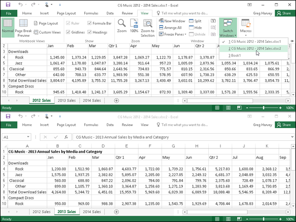
Figure 4-11: Using windows to compare data stored on two different sheets in the same workbook.
As you can see, the top window shows the upper-left portion of the first worksheet with the 2012 sales data, while the lower window shows the upper-left portion of the second worksheet with the 2013 sales data. Note that both windows contain the same sheet tabs (although different tabs are active in the different windows) but that only the top, active window is equipped with a set of horizontal and vertical scroll bars. However, because Excel automatically synchronizes the scrolling between the windows, you can use the single set of scroll bars to bring different sections of the two sheets into view.
Here is the procedure I followed to create and arrange these windows in the CG Music 2012 – 2014 Sales.xlsx workbook:
Open the workbook file for editing and then create a new window by clicking the New Window command button on the View tab of the Ribbon — you can also do this by pressing Alt+WN.
Excel appends the number 2 to the workbook’s filename displayed at the top of the screen (as in CG Music 2012 – 2014 Sales.xlsx:2) to indicate that a new window has been added to the workbook.
- Arrange the windows one on top of the other by clicking the View Side by Side command button (the one with the pages side by side to the immediate right of the Split button) in the Window group of the View tab or by pressing Alt+WB.
- Click the lower window (indicated by the “:2” after the filename on its title bar) to activate the window and then click the 2013 Sales sheet tab to activate it and the Unpin the Ribbon button to display only Ribbon tabs in the first window.
- Click the upper window (indicated by the “:1” following the filename on its title bar) to activate the window and then click its Collapse the Ribbon button to display only Ribbon tabs in the second window.
You can also switch between windows open in a workbook by clicking the Switch Windows button on the View tab followed by the name (with number) of the window you want to activate.
Immediately below the View Side by Side command button in the Windows group on the View tab of the Ribbon, you find these two command buttons:
- Synchronous Scrolling: When this button is selected, any scrolling that you do in the worksheet in the active window is mirrored and synchronized in the worksheet in the inactive window beneath it. To be able to scroll the worksheet in the active window independently of the inactive window, click the Synchronous Scrolling button to deactivate it.
- Reset Window Position: Click this button if you manually resize the active window (by dragging its size box) and then want to restore the two windows to their previous side-by-side arrangement.
To remove the side-by-side windows, click the View Side by Side command button again or press Alt+WB. Excel returns the windows to the display arrangement selected (see “Window arrangements” that follows for details) before clicking the View Side by Side command button the first time. If you haven’t previously selected a display option in the Arrange Windows dialog box, Excel displays the active window full size.
Note that you can use the View Side by Side feature when you have more than two windows open on a single workbook. When three or more windows are open at the time you click the View Side by Side command button, Excel opens the Compare Side by Side dialog box. This dialog box displays a list of all the other open windows with which you can compare the active one. When you click the name of this window and click OK in the Compare Side by Side dialog box, Excel places the active window above the one you just selected (using the arrangement shown in Figure 4-11).
Note, too, that you can use Excel’s View Side by Side feature to compare worksheets in different workbooks just as well as different sheets in the same workbook. (See “Comparing windows on different workbooks” later in this chapter.)
Window arrangements
After creating one or more additional windows for a workbook (by clicking the New Window command button on the View tab), you can then vary their arrangement by selecting different arrangement options in the Arrange Windows dialog box, opened by clicking the Arrange All button on the View tab (or by pressing Alt+WA). The Arrange Windows dialog box contains the following four Arrange options:
- Tiled: Select this option button to have Excel arrange and size the windows so that they all fit side by side on the screen in the order in which you open them (when only two windows are open, selecting the Tiled or Vertical option results in the same side-by-side arrangement).
- Horizontal: Select this option button to have Excel size the windows equally and then place them one above the other (this is the default arrangement option that Excel uses when you click the View Side by Side command button).
- Vertical: Select this option button to have Excel size the windows equally and then place them next to one other, vertically from left to right.
- Cascade: Select this option button to have Excel arrange and size the windows so that they overlap one another with only their title bars visible.
After arranging your windows, you can then select different sheets to display in either window by clicking their sheet tabs, and you can select different parts of the sheet to display by using the window’s scroll bars.
To activate different windows on the workbook so that you can activate a different worksheet by selecting its sheet tab and/or use the scroll bars to bring new data into view, click the window’s title bar or press Ctrl+F6 until its title bar is selected.
When you want to resume normal, full-screen viewing in the workbook window, click the Maximize button in one of the windows. To get rid of a second window, click its button on the taskbar and then click its Close Window button on the far right side of the menu bar (the one with the X). (Be sure that you don’t click the Close button on the far-right of the Excel title bar, because doing this closes your workbook file and exits you from Excel!)
Working with Multiple Workbooks
Working with more than one worksheet in a single workbook is bad enough, but working with worksheets in different workbooks can be really wicked. The key to doing this successfully is just keeping track of “who’s on first”; you do this by opening and using windows on the individual workbook files you have open.
With the different workbook windows in place, you can then compare the data in different workbooks, use the drag-and-drop method to copy or move data between workbooks, or even copy or move entire worksheets.
Comparing windows on different workbooks
To work with sheets from different workbook files you have open, you manually arrange their workbook windows in the Excel Work area, or you click the View Side by Side command button on the View tab of the Ribbon or press Alt+WB. If you have only two workbooks open when you do this, Excel places the active workbook that you last opened above the one that opened earlier (with their active worksheets displayed). If you have more than two workbooks open, Excel displays the Compare Side by Side dialog box where you click the name of the workbook that you want to compare with the active one.
If you need to compare more than two workbooks on the same screen, instead of clicking the View Side by Side button on the View tab, you click the Arrange All button and then select the desired Arrange option (Tiled, Horizontal, Vertical, or Cascading) in the Arrange Windows dialog box. Just make sure when selecting this option that the Windows of Active Workbook check box is not selected in the Arrange Windows dialog box.
Transferring data between open windows
After the windows on your different workbooks are arranged onscreen the way you want them, you can compare or transfer information between them. To compare data in different workbooks, you switch between the different windows, activating and bringing the regions of the different worksheets you want to compare into view.
To move data between workbook windows, arrange the worksheets in these windows so that both the cells with the data entries you want to move and the cell range into which you want to move them are both displayed in their respective windows. Then, select the cell selection to be moved, drag it to the other worksheet window, drag it to the first cell of the range where it is to be moved to, and release the mouse button. To copy data between workbooks, you follow the exact same procedure, except that you hold down the Ctrl key as you drag the selected range from one window to another. (See Book II, Chapter 3 for information on using drag-and-drop to copy and move data entries.)
When you’re finished working with workbook windows arranged in some manner in the Excel Work area, you can return to the normal full-screen view by clicking the Maximize button on one of the windows. As soon as you maximize one workbook window, all the rest of the arranged workbook windows are made full size as well. If you used the View Side by Side feature to set up the windows, you can do this by clicking the View Side by Side command button on the View tab again or by pressing Alt+WB.
Transferring sheets from one workbook to another
Instead of copying cell ranges from one workbook to another, you can move (or copy) entire worksheets between workbooks. You can do this with drag-and-drop or by choosing the Move or Copy Sheet option from the Format command button’s drop-down menu on the Ribbon’s Home tab.
To use drag-and-drop to move a sheet between open windows, you simply drag its sheet tab from its window to the place on the sheet tabs in the other window where the sheet is to be moved to. As soon as you release the mouse button, the entire worksheet is moved from one file to the other, and its sheet tab now appears among the others in that workbook. To copy a sheet rather than move it, you perform the same procedure, except that you hold down the Ctrl key as you drag the sheet tab from one window to the next.
To use the Move or Copy Sheet option on the Format command button’s drop-down menu to move or copy entire worksheets, you follow these steps:
Open both the workbook containing the sheets to be moved or copied and the workbook where the sheets will be moved or copied to.
Both the source and destination workbooks must be open in order to copy or move sheets between them.
Click the workbook window with sheets to be moved or copied.
Doing this activates the source workbook so that you can select the sheet or sheets you want to move or copy.
Select the sheet tab of the worksheet or worksheets to be moved or copied.
To select more than one worksheet, hold down the Ctrl key as you click the individual sheet tabs.
Click the Format button on the Home tab and then choose Move or Copy Sheet from the drop-down menu or press Alt+HOM.
Doing this opens the Move or Copy dialog box, as shown in Figure 4-12.
From the To Book drop-down menu, choose the filename of the workbook into which the selected sheets are to be moved or copied.
If you want to move or copy the selected worksheets into a new workbook file, choose the (New Book) item at the very top of this drop-down menu.
In the Before Sheet list box, click the name of the sheet that should immediately follow the sheet(s) that you’re about to move or copy into this workbook.
If you want to move or copy the selected sheet(s) to the very end of the destination workbook, click (Move to End) at the bottom of this list box.
If you want to copy the selected sheet(s) rather than move them, select the Create a Copy check box.
If you don’t select this check box, Excel automatically moves the selected sheet(s) from one workbook to the other instead of copying them.
- Click OK to close the Move or Copy dialog box and complete the move or copy operation.
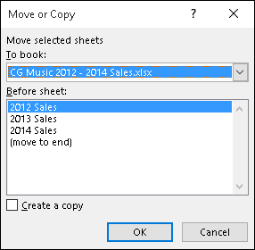
Figure 4-12: Copying a worksheet to another workbook using the Move or Copy dialog box.
Consolidating Worksheets
Excel allows you to consolidate data from different worksheets into a single worksheet. Using the program’s Consolidate command button on the Data tab of the Ribbon, you can easily combine data from multiple spreadsheets. For example, you can use the Consolidate command to total all budget spreadsheets prepared by each department in the company or to create summary totals for income statements for a period of several years. If you used a template to create each worksheet you’re consolidating, or an identical layout, Excel can quickly consolidate the values by virtue of their common position in their respective worksheets. However, even when the data entries are laid out differently in each spreadsheet, Excel can still consolidate them provided that you’ve used the same labels to describe the data entries in their respective worksheets.
Most of the time, you want to total the data that you’re consolidating from the various worksheets. By default, Excel uses the SUM function to total all the cells in the worksheets that share the same cell references (when you consolidate by position) or that use the same labels (when you consolidate by category). You can, however, have Excel use any of other following statistical functions when doing a consolidation: AVERAGE, COUNT, COUNTA, MAX, MIN, PRODUCT, STDEV, STDEVP, VAR, or VARP. (See Book III, Chapter 5 for more information on these functions.)
To begin consolidating the sheets in the same workbook, you select a new worksheet to hold the consolidated data. (If need be, insert a new sheet in the workbook by clicking the Insert Worksheet button.) To begin consolidating sheets in different workbooks, open a new workbook. If the sheets in the various workbooks are generated from a template, open the new workbook for the consolidated data from that template.
Before you begin the consolidation process on the new worksheet, you choose the cell or cell range in this worksheet where the consolidated data is to appear. (This range is called the destination area.) If you select a single cell, Excel expands the destination area to columns to the right and rows below as needed to accommodate the consolidated data. If you select a single row, the program expands the destination area down subsequent rows of the worksheet, if required to accommodate the data. If you select a single column, Excel expands the destination area across columns to the right, if required to accommodate the data. If, however, you select a multi-cell range as the destination area, the program does not expand the destination area and restricts the consolidated data just to the cell selection.
If you want Excel to use a particular range in the worksheet for all consolidations you perform in a worksheet, assign the range name Consolidate_Area to this cell range. Excel then consolidates data into this range whenever you use the Consolidate command.
When consolidating data, you can select data in sheets in workbooks that you’ve opened in Excel or in sheets in unopened workbooks stored on disk. The cells that you specify for consolidation are referred to as the source area, and the worksheets that contain the source areas are known as the source worksheets.
If the source worksheets are open in Excel, you can specify the references of the source areas by pointing to the cell references (even when the Consolidate dialog box is open, Excel will allow you to activate different worksheets and scroll through them as you select the cell references for the source area). If the source worksheets are not open in Excel, you must type in the cell references as external references, following the same guidelines you use when typing a linking formula with an external reference (except that you don’t type =). For example, to specify the data in range B4:R21 on Sheet1 in a workbook named CG Music - 2014 Sales.xlsx as a source area, you enter the following external reference:
'[CG Music – 2014 Sales.xlsx]Sheet1'!$b$4:$r$21
Note that if you want to consolidate the same data range in all the worksheets that use a similar filename (for example, CG Music - 2012 Sales, CG Music - 2013 Sales, CG Music - 2014 Sales, and so on), you can use the asterisk (*) or the question mark (?) as wildcard characters to stand for missing characters as in
'[CG Music - 20?? Sales.xlsx]Sheet1'!$B$4:$R$21
In this example, Excel consolidates the range A2:R21 in Sheet1 of all versions of the workbooks that use “CG - Music - 20” in the main file when this name is followed by another two characters (be they 12, 13, 14, 15, and so on).
When you consolidate data, Excel uses only the cells in the source areas that contain values. If the cells contain formulas, Excel uses their calculated values, but if the cells contain text, Excel ignores them and treats them as though they were blank (except in the case of category labels when you’re consolidating your data by category as described later in this chapter).
Consolidating by position
You consolidate worksheets by position when they use the same layout (such as those created from a template). When you consolidate data by position, Excel does not copy the labels from the source areas to the destination area, only values. To consolidate worksheets by position, you follow these steps:
Open all the workbooks with the worksheets you want to consolidate. If the sheets are all in one workbook, open it in Excel.
Now you need to activate a new worksheet to hold the consolidated data. If you’re consolidating the data in a new workbook, you need to open it (File ⇒ New or Alt+FN). If you’re consolidating worksheets generated from a template, use the template to create the new workbook in which you are to consolidate the spreadsheet data.
Open a new worksheet to hold the consolidated data (Ctrl+N).
Next, you need to select the destination area in the new worksheet that is to hold the consolidated data.
Click the cell at the beginning of the destination area in the consolidation worksheet, or select the cell range if you want to limit the destination area to a particular region.
If you want Excel to expand the size of the destination area as needed to accommodate the source areas, just select the first cell of this range.
Click the Consolidate command button on the Data tab of the Ribbon or press Alt+AN.
Doing this opens the Consolidate dialog box similar to the one shown in Figure 4-13. By default, Excel uses the SUM function to total the values in the source areas. If you want to use another statistical function such as AVERAGE or COUNT, select the desired function from the Function drop-down list box.
(Optional) Select the function you want to use from the Function drop-down list box if you don’t want the values in the source areas summed together.
Now, you need to specify the various source ranges to be consolidated and add them to the All References list box in the Consolidate dialog box. To do this, you specify each range to be used as the source data in the Reference text box and then click the Add button to add it to the All References list box.
Select the cell range or type the cell references for the first source area in the Reference text box.
When you select the cell range by pointing, Excel minimizes the Consolidate dialog box to the Reference text box so that you can see what you’re selecting. If the workbook window is not visible, choose it from the Switch Windows button on the View tab or the Windows taskbar and then select the cell selection as you normally would. (Remember that you can move the Consolidate dialog box minimized to the Reference text box by dragging it by the title bar.)
If the source worksheets are not open, you can click the Browse command button to select the filename in the Browse dialog box to enter it (plus an exclamation point) into the Reference text box, and then you can type in the range name or cell references you want to use. If you prefer, you can type in the entire cell reference including the filename. Remember that you can use the asterisk (*) and question mark (?) wildcard characters when typing in the references for the source area.
- Click the Add command button to add this reference to the first source area to the All References list box.
- Repeat Steps 6 and 7 until you have added all the references for all the source areas that you want to consolidate.
- Click the OK button in the Consolidate dialog box.
Excel closes the Consolidate dialog box and then consolidates all the values in the source areas in the place in the active worksheet designated as the destination area. Note that you can click the Undo button on the Quick Access toolbar or press Ctrl+Z to undo the effects of a consolidation if you find that you defined the destination and/or the source areas incorrectly.
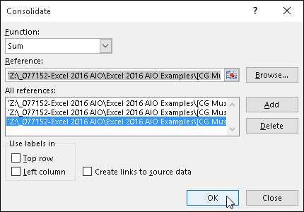
Figure 4-13: Using the Consolidate dialog box to total sales data for three years stored on separate worksheets.
Figure 4-14 shows you the first part of a consolidation for three years (2012, 2013, and 2014) of record store sales in the newly created CG Music 2012 - 2014 Consolidated Sales.xlsx file in the workbook window in the upper-left corner. The Consolidated worksheet in this file totals the source area B4:R21 from the Sales worksheets in the CG Music - 2012 Sales.xlsx workbook with the 2012 annual sales, the CG Music - 2013 Sales.xlsx workbook with the 2013 annual sales, and the CG Music - 2014 Sales.xlsx workbook with the 2014 annual sales. These sales figures are consolidated in the destination area, B4:R21, in the Consolidated sheet in the CG Music 2012 - 2014 Consolidated Sales.xls workbook. (However, because all these worksheets use the same layout, only cell B4, the first cell in this range, was designated at the destination area.)
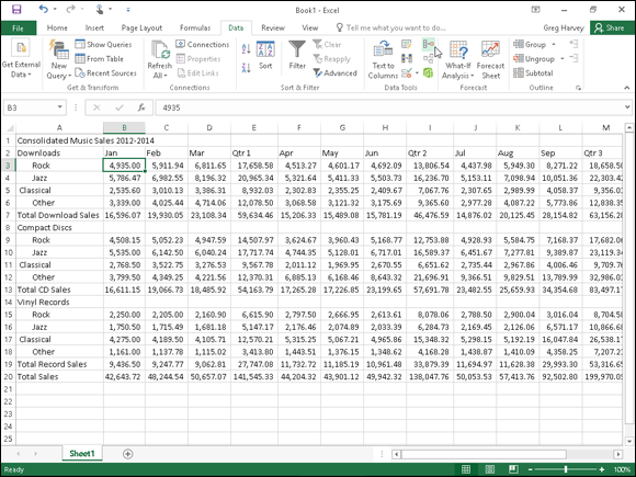
Figure 4-14: The Consolidated worksheet after having Excel total sales from the last three years.
Excel allows only one consolidation per worksheet at one time. You can, however, add to or remove source areas and repeat a consolidation. To add new source areas, open the Consolidate dialog box and then specify the cell references in the Reference text box and click the Add button. To remove a source area, click its references in the All References list box and then click the Delete button. To perform the consolidation with the new source areas, click OK. To perform a second consolidation in the same worksheet, choose a new destination area, open the Consolidate dialog box, clear all the source areas you don’t want to use in the All References list box with the Delete button, and then redefine all the new source areas in the Reference text box with the Add button before you perform the consolidation by clicking the OK button.
Consolidating by category
You consolidate worksheets by category when their source areas do not share the same cell coordinates in their respective worksheets, but their data entries do use common column and/or row labels. When you consolidate by category, you include these identifying labels as part of the source areas. Unlike when consolidating by position, Excel copies the row labels and/or column labels when you specify that they should be used in the consolidation.
When consolidating spreadsheet data by category, you must specify whether to use the top row of column labels and/or the left column of row labels in determining which data to consolidate. To use the top row of column labels, you select the Top Row check box in the Use Labels In section of the Consolidate dialog box. To use the left column of row labels, you select the Left Column check box in this area. Then, after you’ve specified all the source areas (including the cells that contain these column and row labels), you perform the consolidation in the destination area by clicking the Consolidate dialog box’s OK button.
Linking consolidated data
Excel allows you to link the data in the source areas to the destination area during a consolidation. That way, any changes that you make to the values in the source area are automatically updated in the destination area of the consolidation worksheet. To create links between the source worksheets and the destination worksheet, you simply select the Create Links to Source Data check box in the Consolidate dialog box to put a check mark in it when defining the settings for the upcoming consolidation.
When you perform a consolidation with linking, Excel creates the links between the source areas and the destination area by outlining the destination area. (See “Outlining worksheets” earlier in this chapter for details.) Each outline level created in the destination area holds rows or columns that contain the linking formulas to the consolidated data.