Chapter 6
Adding Formulas to Power Pivot
In This Chapter
![]() Creating, formatting, and hiding your own calculated columns
Creating, formatting, and hiding your own calculated columns
![]() Creating calculated columns by using DAX
Creating calculated columns by using DAX
![]() Creating calculated measures
Creating calculated measures
![]() Breaking out of pivot tables with cube functions
Breaking out of pivot tables with cube functions
When analyzing data with Power Pivot, you often find the need to expand your analysis to include data based on calculations that are not in the original dataset. Power Pivot has a robust set of functions (called DAX functions) that allow you to perform mathematical operations, recursive calculations, data lookups, and much more.
This chapter introduces you to DAX functions and provides the ground rules for building your own calculations in Power Pivot data models.
Enhancing Power Pivot Data with Calculated Columns
Calculated columns are columns you create to enhance a Power Pivot table with your own formulas. When you enter calculated columns directly in the Power Pivot window, they become part of the source data you use to feed your pivot table. Calculated columns work at the row level. That is to say, the formulas you create in a calculated column perform their operations based on the data in each individual row. For example, if you have a Revenue column and a Cost column in your Power Pivot table, you could create a new column that calculates [Revenue] minus [Cost]. This simple calculation is valid for each row in the data set.
Calculated measures are used to perform more complex calculations that work on an aggregation of data. These calculations are applied directly to a pivot table, creating a sort of virtual column that can’t be seen in the Power Pivot window. Calculated measures are needed whenever you need to calculate based on an aggregated grouping of rows — for example, the sum of [Year2] minus the sum of [Year1].
Creating your first calculated column
Creating a calculated column works much like building formulas in an Excel table. Follow these steps to create a calculated column:
Activate the Power Pivot window (click the Manage command button on the Power Pivot Ribbon tab), and then select the Invoice Details tab.
In the table, you see an empty column on the far right, labeled Add Column.
- Click on the first blank cell in that column.
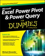
- On the Formula bar, enter the following formula (as shown in Figure 6-1):
=[UnitPrice]*[Quantity] Press Enter.
The formula populates the entire column, and Power Pivot automatically renames the column to Calculated Column 1.
Double-click on the column label and rename the column Total Revenue.
 You can rename any column in the Power Pivot window by double-clicking the column name and entering a new name. Alternatively, you can right-click any column and choose the Rename option.
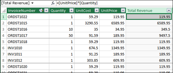
Figure 6-1: Start the calculated column by entering an operation on the Formula bar.
You can build calculated columns by clicking instead of typing. For example, rather than manually enter =[UnitPrice]*[Quantity], you can enter the equal sign (=), click the UnitPrice column, type the asterisk (*), and then click the Quantity column. You can also enter your own static data. For example, you can enter a formula to calculate a 10-percent tax rate by entering =[UnitPrice]*1.10.
Each calculated column you create is automatically available in any pivot table connected to the Power Pivot Data Model. You don’t have to take any action to get your calculated columns into the pivot table. Figure 6-2 shows the Total Revenue calculated column in the PivotTable Fields List. These calculated columns can be used just as you would use any other field in the pivot table.
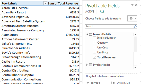
Figure 6-2: Calculated columns automatically show up in the PivotTable Fields List.
If you need to edit the formula in a calculated column, find the calculated column in the Power Pivot window, click the column, and then make changes directly on the Formula bar.
See Chapter 2 for a refresher on how to create a pivot table from Power Pivot.
Formatting calculated columns
You often need to change the formatting of Power Pivot columns to appropriately match the data within them. For example, you may want to show numbers as currency, remove decimal places, or display dates in a certain way.
You’re by no means limited to formatting only calculated columns. The following steps can be used to format any column you see in the Power Pivot window:
- In the Power Pivot window, click on the column you want to format.
- Go to the Home tab of the Power Pivot window and find the Formatting group (see Figure 6-3).
- Use the option to alter the formatting of the column as you see fit.
Figure 6-3: You can use the formatting tools found on the Power Pivot window’s Home tab to format any column in the Data Model.
Veteran Excel pivot table users know that changing pivot table number formats one data field at a time is a pain. One fantastic feature of Power Pivot formatting is that any format you apply to the columns in the Power Pivot window is automatically applied to all pivot tables connected to the Data Model.
Referencing calculated columns in other calculations
As with all calculations in Excel, Power Pivot allows you to reference a calculated column as a variable in another calculated column. Figure 6-4 illustrates this concept with a new calculated column named Gross Margin. Notice that on the Formula bar, the calculation is using the [Total Revenue] calculated column that you create earlier in this chapter.
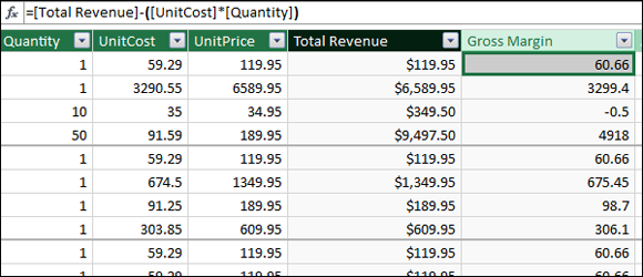
Figure 6-4: The new Gross Margin calculation is using the previously created [Total Revenue] and calculated column.
Hiding calculated columns from end users
Because calculated columns can reference each other, you can imagine creating columns simply as helper columns for other calculations. You may not want your end users to see these columns in your client tools. (In this context, client tools refers to pivot tables, Power View dashboards, and Power Map.)
Similar to hiding columns on an Excel worksheet, Power Pivot allows you to hide any column. (It doesn’t have to be a calculated column.) To hide columns, select the columns you want hidden, right-click the selection, and then choose the Hide from Client Tools option (as shown in Figure 6-5).
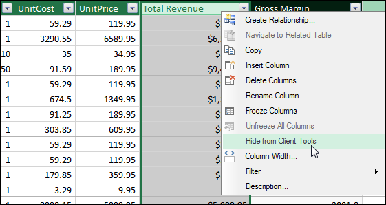
Figure 6-5: Right-click and select Hide from Client Tools.
 When a column is hidden, it doesn’t show as an available selection in the PivotTable Fields List. However, if the column you’re hiding is already part of the pivot report (meaning you’ve already dragged it onto the pivot table), hiding the column doesn’t automatically remove it from the report. Hiding merely affects the ability to see the column in the PivotTable Fields List.
Note in Figure 6-6 that Power Pivot recolors columns based on their attributes. Hidden columns are subdued and grayed-out, whereas calculated columns that are not hidden have a darker (black) header.
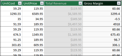
Figure 6-6: Hidden columns are grayed-out, and calculated columns have darker headings.
To unhide columns, select the hidden columns in the Power Pivot window, right-click on the selection, and then choose the Unhide from Client Tools option.
Utilizing DAX to Create Calculated Columns
Data Analysis Expressions, or DAX, is essentially the formula language that Power Pivot uses to perform calculations within its own construct of tables and columns. The DAX formula language comes supplied with its own set of functions. Some of these functions can be used in calculated columns for row-level calculations, and others are designed to be used in calculated measures to aggregate operations.
In this section, I touch on some of the DAX functions that you can leverage in calculated columns.
DAX has more than 150 different functions. The examples of DAX that I demonstrate in this chapter are meant to give you a sense of how calculated columns and calculated measures work. A full overview of DAX is beyond the scope of this book. If, after reading this chapter, you want to read more about DAX, however, pick up The Definitive Guide to DAX, by Alberto Ferrari and Marco Russo. Ferrari and Russo provide an excellent overview of DAX that is comprehensive but easy to understand.
Identifying DAX functions that are safe for calculated columns
Earlier in this chapter, you use the Formula bar within the Power Pivot window to enter calculations. Next to the Formula bar, you may have noticed the Insert Function button: the button labeled fx. It’s similar to the Insert Function button in Excel. Clicking this button opens the Insert Function dialog box, shown in Figure 6-7. Using this dialog box, you can browse, search for, and insert the available DAX functions.
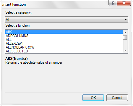
Figure 6-7: The Insert Function dialog box shows you all available DAX functions.
As you look through the list of DAX functions, notice that many of them look like the common Excel functions that most people are familiar with. But make no mistake: They aren’t Excel functions. Whereas Excel functions work with cells and ranges, these DAX functions are designed to work at the table and column levels.
To understand what I mean, start a new calculated column on the Invoice Details tab. Click on the Formula bar and type a good old SUM function: SUM([Gross Margin]). The result is shown in Figure 6-8.
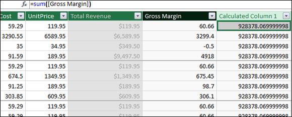
Figure 6-8: The DAX SUM function can only sum the column as a whole.
As you can see, the SUM function sums the entire column. This is because Power Pivot and DAX are designed to work with tables and columns. Power Pivot has no construct for cells and ranges. It doesn’t even have column letters and row numbers on its grid. Though you would normally reference a range (as in an Excel SUM function), DAX basically takes the entire column.
The bottom line is that not all DAX functions can be used with calculated columns. Because a calculated column evaluates at the row level, only DAX functions that evaluate single data points can be used in a calculated column.
Here’s a good rule of thumb: If the function requires an array or a range of cells as an argument, it isn’t viable in a calculated column.
So, functions such as SUM, MIN, MAX, AVERAGE, and COUNT don’t work in calculated columns. Functions that require only single data-point arguments work quite well in calculated columns: functions such as YEAR, MONTH, MID, LEFT, RIGHT, IF, and IFERROR.
Building DAX-driven calculated columns
To demonstrate the usefulness of employing a DAX function to enhance calculated columns, let’s return to the walk-through example. Go to the Power Pivot window and select the InvoiceHeader tab on the Ribbon. If you’ve accidentally closed the Power Pivot window, you can open it by clicking the Manage command button on the Power Pivot Ribbon tab.
The InvoiceHeader tab, shown in Figure 6-9, contains an InvoiceDate column. Although this column is valuable in the raw table, the individual dates aren’t convenient when analyzing the data with a pivot table. It would be beneficial to have a column for Month and a column for Year. This way, you could aggregate and analyze the data by month and year.
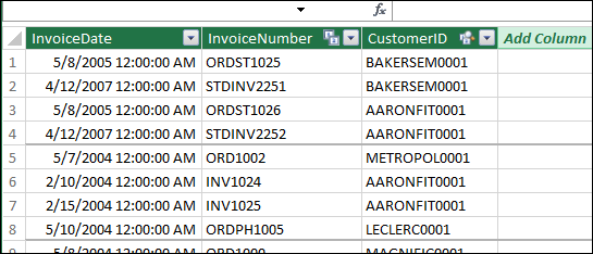
Figure 6-9: DAX functions can help enhance the invoice header data with Year and Month time dimensions.
For this endeavor, you use the DAX functions YEAR( ), MONTH( ), and FORMAT( ) to add some time dimensions to the Data Model. Follow these steps:
- In the InvoiceHeader table, click on the first blank cell in the empty column labeled Add Column, on the far right.
On the Formula bar, type =YEAR([InvoiceDate]) and then press Enter.
Power Pivot automatically renames the column to Calculated Column 1.
- Double-click on the column label and rename the column Year.
- Starting in the next column, click on the first blank cell in the empty column labeled Add Column, on the far right.
On the Formula bar, type =MONTH([InvoiceDate]), and then press Enter.
Power Pivot automatically renames the column to Calculated Column 1.
- Double-click on the column label and rename the column Month.
- Starting in the next column, click on the first blank cell in the empty column labeled Add Column, on the far right.
On the Formula bar, type =FORMAT([InvoiceDate],”mmm”) and then press Enter.
Power Pivot automatically renames the column to Calculated Column 1.
- Double-click on the column label and rename the column Month Name.
After completing these steps, you should have three new calculated columns similar to the ones shown in Figure 6-10.
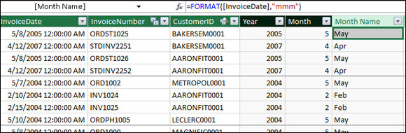
Figure 6-10: Using DAX functions to supplement a table with Year, Month, and Month Name columns.
As I mention earlier in this chapter, creating calculated columns automatically makes them available through the PivotTable Fields List (see Figure 6-11).
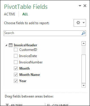
Figure 6-11: DAX calculations are immediately available in any connected pivot table.
One of the more annoying aspects of Power Pivot is that it doesn’t inherently know how to sort months. Unlike standard Excel, Power Pivot doesn’t use the built-in custom lists that define the order of month names. Whenever you create a calculated column such as [Month Name] and place it into your pivot table, Power Pivot puts those months in alphabetical order, as shown in Figure 6-12.
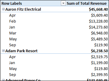
Figure 6-12: Month names in Power Pivot-driven pivot tables don’t automatically sort in month order.
The fix for this problem is fairly easy. Open the Power Pivot window and select the Home tab. There, click the Sort by Column command button. The Sort by Column dialog box the opens, as shown in Figure 6-13.
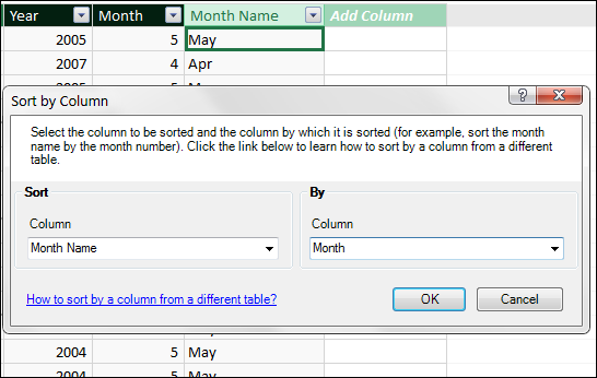
Figure 6-13: The Sort by Column dialog box lets you define how columns are sorted.
The idea is to select the column you want sorted and then select the column you want to sort by. In this scenario, you want to sort Month Name by month.
After you confirm the change, it initially appears as though nothing has happened. The reason is that the sort order you defined isn’t for the Power Pivot window. The sort order is applied to the pivot table. You can switch over to Excel to see the result in the pivot table (see Figure 6-14).
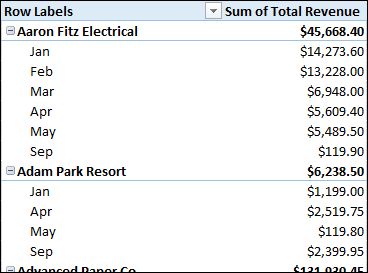
Figure 6-14: The month names now show in the correct month order.
Referencing fields from other tables
Sometimes, the operation you’re trying to perform with a calculated column requires you to utilize fields from other tables within the Power Pivot Data Model. For example, you may need to account for a customer-specific discount amount from the Customers table (see Figure 6-15) when creating a calculated column in the InvoiceDetails table.
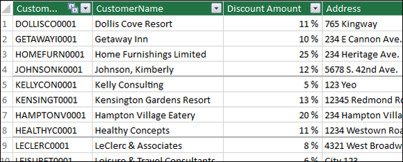
Figure 6-15: The discount amount in the Customers table can be used in a calculated column in another table.
To accomplish this, you can use a DAX function named RELATED. Similar to VLOOKUP in standard Excel, the RELATED function allows you to look up values from one table in order to use them in another.
Follow these steps to create a new calculated column that displays a discounted amount for each transaction in the InvoiceDetails table:
- In the InvoiceDetails table, click on the first blank cell in the empty column labeled Add Column, on the far right.
On the Formula bar, type =RELATED(.
As soon as you enter the open parenthesis, a menu of available fields (shown in Figure 6-16) is displayed. Note that the items in the list represent the table name followed by the field name in brackets. In this case, you’re interested in the Customers[Discount Amount] field.
The RELATED function leverages the relationships you defined when creating the Data Model in order to perform the lookup. So this list of choices contains only the fields that are available based on the relationships you defined.Double-click the Customers[Discount Amount] field and then press Enter.
Power Pivot automatically renames the column to Calculated Column 1.
- Double-click on the column label and rename the column Discount%.
- Starting in the next column, click on the first blank cell in the empty column labeled Add Column, on the far right.
On the Formula bar, type =[UnitPrice]*[Quantity]*(1-[Discount%]) and then press Enter.
Power Pivot automatically renames the column to Calculated Column 1.
- Double-click on the column label and rename the column Discounted Revenue.
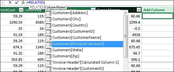
Figure 6-16: Use the RELATED function to look up a field from another table.
The reward for your efforts is a new column that uses the discount percent from the Customers table to calculate discounted revenue for each transaction. Figure 6-17 illustrates the new calculated column.
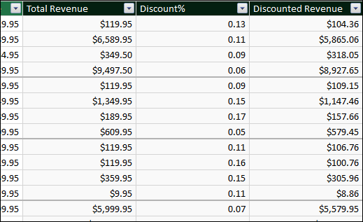
Figure 6-17: The final discount amount calculated column using the Discount% column from the Customers table.
In the example from the preceding section, you first create a Discount% column using the RELATED function, and then you use that column in another calculated column to calculate the discount amount.
You don’t necessarily have to create multiple calculated columns to accomplish a task like this one. You could instead nest the RELATED function into the discount amount calculation. The following line shows the syntax for the nested calculation:
=[UnitPrice]*[Quantity]*
(1-RELATED(Customers[Discount Amount]))
As you can see, nesting simply means to embed functions within a calculation. In this case, rather than use the RELATED function in a separate Discount% field, you can embed it directly into the discounted revenue calculation.
Nesting functions can definitely save time and even improve performance in larger data models. On the other hand, complicated nested functions can be harder to read and understand.
Understanding Calculated Measures
You can enhance the functionality of your Power Pivot reports by using a kind of calculation called a calculated measure. Calculated measures are not applied to the Power Pivot window like calculated columns. Instead, they’re applied directly to the pivot table, creating a sort of virtual column that isn’t visible in the Power Pivot window. You use calculated measures when you need to calculate based on an aggregated grouping of rows.
Creating a calculated measure
Imagine that you want to show the difference in unit costs between the years 2007 and 2006 for each of your customers. Think about what technically has to be done to achieve this calculation: You have to figure out the sum of unit costs for 2007, determine the sum of unit costs for 2006, and then subtract the sum of 2007 from the sum of 2006. This calculation simply can’t be completed using calculated columns. Using calculated measures is the only way to calculate the cost variance between 2007 and 2006.
Follow these steps to create a calculated measure:
Start with a pivot table created from a Power Pivot Data Model.
The Chapter 6 Sample File.xlsx workbook contains the Calculated Measures tab with a pivot table already created.Click the Power Pivot tab on the Excel Ribbon, and choose Measures ⇒ New Measure.
This step opens the Measure dialog box, shown in Figure 6-18.
- In the Measure dialog box, set the following inputs:
- Table name: Choose the table you want to contain the calculated measure when looking at the PivotTable Fields List. Don’t sweat this decision too much. The table you select has no bearing on how the calculation works. It’s simply a preference on where you want to see the new calculation within the PivotTable Fields List.
- Measure name: Give the calculated measure a descriptive name.
- Description: Enter a friendly description to document what the calculation does.
Formula: Enter the DAX formula that will calculate the results of the new field.
In this example, you use the following DAX formula:
=CALCULATE(SUM(InvoiceDetails[UnitCost]),YEAR(InvoiceHeader[InvoiceDate])=2007)This formula uses the CALCULATE function to sum the Total Revenue column from the InvoiceDetails table, where the Year column in the InvoiceHeader is equal to 2007.
- Formatting Options: Specify the formatting for the calculated measure results.
Click the Check Formula button to ensure that there are no syntax errors.
If your formula is well formed, you see the message No errors in formula. If the formula has errors, you see a full description.
Click the OK button to confirm the changes and close the dialog box.
You see your newly created calculated measure in the pivot table.
- Repeat Steps 2–5 for any other calculated measure you need to create.
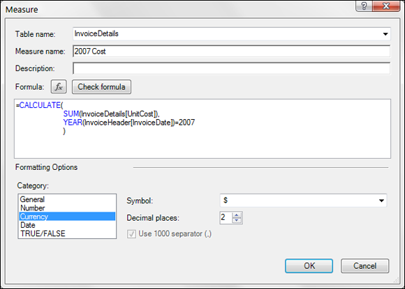
Figure 6-18: Creating a new calculated measure.
In this example, you need a measure to show the 2006 cost:
=CALCULATE(
SUM(InvoiceDetails[UnitCost]),
YEAR(InvoiceHeader[InvoiceDate])=2006
)
You also need a measure to calculate the variance:
=[2007 Revenue]-[2006 Revenue]
Figure 6-19 illustrates the newly created calculated measures. The calculated measures are applied to each customer, displaying the variance between their 2007 and 2006 costs. As you can see, each calculated measure is available for selection in the PivotTable Fields List.
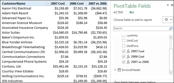
Figure 6-19: Calculated measures can be seen in the PivotTable Fields List.
Always attempt to achieve readability by using carriage returns and spaces. In Figure 6-18, the DAX calculation is entered with carriage returns and spaces. This is purely for readability purposes. DAX ignores white spaces and isn’t case sensitive, so it’s quite forgiving on how you structure the calculation.
Editing and deleting calculated measures
You may find that you need to either edit or delete a calculated measure. You can do so by following these steps:
Click anywhere inside the pivot table, click the Power Pivot tab on the Excel Ribbon, and choose Measures ⇒ Manage Measures.
This step opens the Manage Measures dialog box, shown in Figure 6-20.
- Select the target calculated measure, and click one of these two buttons:
- Edit: Opens the Measure dialog box, where you can make changes to the calculation setting.
- Delete: Opens a message box asking you to confirm that you want to remove the measure. After you confirm, the calculated measure is removed.
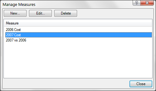
Figure 6-20: The Manage Measures dialog box lets you edit or delete your calculated measures.
Free Your Data With Cube Functions
Cube functions are Excel functions that can be used to access the data in a Power Pivot Data Model outside the constraints of a pivot table. Although cube functions aren’t technically used to create calculations themselves, they can be used to free PowerPivot data so that it can be used with formulas you may have in other parts of your Excel spreadsheet.
One of the easiest ways to start exploring cube functions is to allow Excel to convert your Power Pivot pivot table into cube functions. The idea is to tell Excel to replace all cells in the pivot table with a formula that connects back to the Power Pivot Data Model.
Follow these steps to create your first set of cube functions:
Start with a pivot table created from a Power Pivot model.
The Chapter 6 Sample File.xlsx workbook contains a Cube Functions tab with a pivot table already created.- Place the cursor anywhere inside the pivot table, and then select Analyze ⇒ Convert to Formulas, as shown in Figure 6-21.
In the Measure dialog box, set the following inputs: Table Name, Measure Name, Formula, and Formatting Options.
After a second or two, the cells that formerly housed a pivot table are now homes for cube formulas. The Formula bar, shown in Figure 6-22, illustrates the cube functions.
If the pivot table contains a report filter field, the dialog box shown in Figure 6-23 opens. This dialog box gives you the option to convert the filter drop-down selectors to cube formulas. If you select this option, the drop-down selectors are removed, leaving a static formula.
If you need to have the filter drop-down selectors intact so you can interactively change the selections in the filter field, leave the Convert Report Filters option deselected.
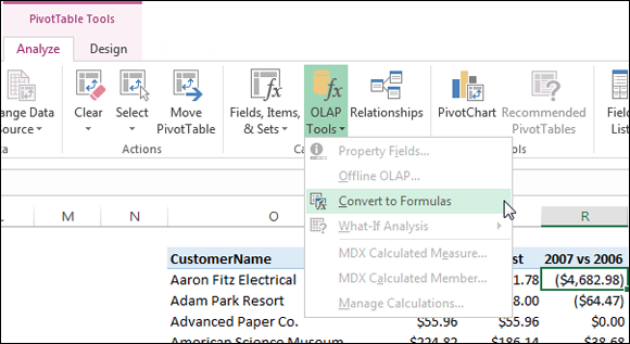
Figure 6-21: Select the Convert to Formulas option to convert the pivot table to cube formulas.
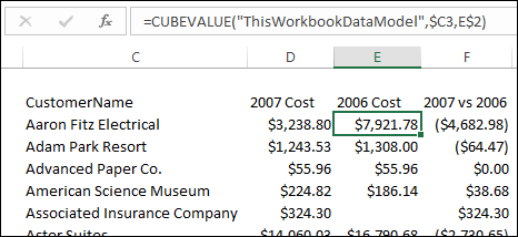
Figure 6-22: These cells are now a series of cube functions!
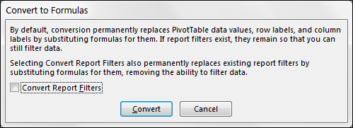
Figure 6-23: Excel gives you the option to convert your report filter fields.
Why is this capability useful? Well, now that the values you see are no longer part of a pivot table object, you can insert rows and columns, add your own calculations, or combine the data with other formulas in your spreadsheet.
The bottom line is that cube functions give you the flexibility to free your Power Pivot data from the confines of a pivot table and then use it in all sorts of ways by simply moving formulas around.