Chapter 7

Backpropagation

7.1 Definition

In Chapter 6, we discussed some aspects of functioning and teaching a single-layer neural network built from nonlinear elements. Let us continue the analysis now, showing how multilayer nonlinear networks work. They present more significant and interesting possibilities, as we saw from working with the Example 06 program.

You now know how to build multilayer networks from nonlinear neurons and how a nonlinear neuron can be taught, for example, by modifying Example 06. However, you have not yet encountered a basic problem of teaching such multilayer neural networks built from nonlinear neurons: the so-called hidden layers (Figure 7.1). What is the impact of this problem?

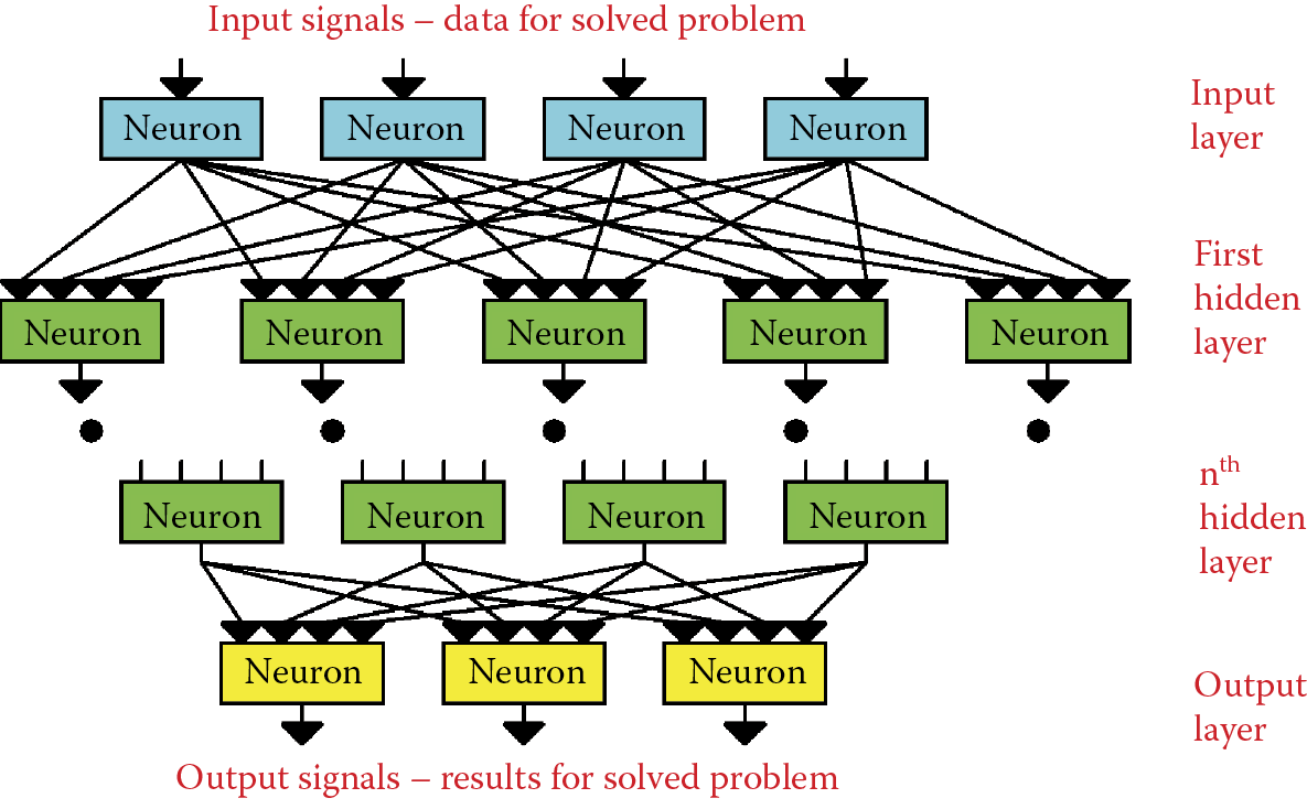
The rules of teaching that you encountered in earlier chapters were based on a simple but very successful method: each neuron of a network individually introduces corrections to its working knowledge by changing the values of the weight coefficients on all its inputs on the basis of a set error value. In a single-layer network, the situation was simple and obvious. The output signal of each neuron was compared with the correct value given by the teacher and this step was sufficient to enable the neuron to correct the weights. The process is not quite as easy for a multilayer network. Neurons of the final (output) layer may have their errors estimated simply by a comparison of the signal produced by each neuron with a model signal from the teacher.

What about the neurons from the previous layers? Their errors must be estimated mathematically because they cannot be measured directly. We do not know what the values of the correct signals should be because the teacher does not define the intermediate values and focuses only on the final result.

A method commonly used to “guess” the errors of neurons in hidden layers is called backpropagation (short for backward propagation). This method is so popular that in most programs used to create networks and teaching networks, backpropagation is applied as default method. Other teaching methods, for example, involve an accelerated method of this algorithm called quick propagation and systems based on sophisticated mathematical methods such as conjugate gradient and Levenberg–Marquardt methods.

Backpropagation methods have the advantage of speed but the advantage is available only when a problem to be solved by a neural network (by finding a solution based on its learning) meets all the sophisticated mathematical requirements. We may know the problem to be solved but have no idea whether it meets the complex requirements.

What does that mean in practice? Assume we have a difficult task to solve. We start teaching a neural network with a sophisticated modern method such as the Levenberg–Marquardt algorithm. If we had the type of problem for which the algorithm was designed, the network could be taught quickly. If the problem does not fit this specification, the algorithm will endlessly lead the network astray because the theoretical assumptions of the algorithm are not met.

The huge advantage of backpropagation is that unlike other techniques, it works independently of theoretical assumptions. While complex clever algorithms sometimes work, backpropagation always works. Its operation may be irritatingly slow but it will never let you down.

You should understand backpropagation because people who work with neural networks rely on it as a dependable partner.

The backpropagation method will be presented through the analysis of the behavior of another program. Before that, however, we must cover one new detail that is very important: the shapes of nonlinear characteristics used in testing neurons.

7.2 Changing Thresholds of Nonlinear Characteristics

Chapter 6 discussed neurons based on the all-or-nothing concept. They were based on logical categorization of input signals (true or false; 1 or 0) or on bipolar characteristics (approval or disapproval; +1 or –1). In both cases the transition between two states was sudden. If the summed output signals exceeded the threshold, the instant result was +1. If the output signals were so weak (a condition known as subliminal stimulation), the system indicated no reaction (0) or a totally negative (–1) reaction.

The rule of zero value of threshold was assumed, which meant that the positive sum of input signals was +1 and the negative value was 0 or –1, and this limited the possibilities of such networks. As we discuss the transitions of nonlinear neurons, keep in mind the value of threshold: it need not have zero value.

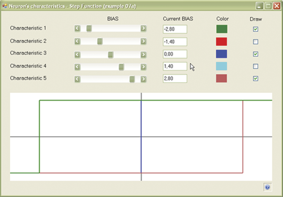
In the nonlinear models of neurons analyzed in this chapter, the threshold will be released. This will lead to the appearance of moving characteristics chosen freely by a feature called BIAS included in programs for modeling networks. The Example 07a program will enable you to understand a family of threshold characteristics of neurons by changing BIAS values. The result will be a good overview of the role of BIAS in shaping the behaviors of single neurons and whole networks. This program demonstrates the behavior of a neuron with a freely shaped threshold (Figure 7.2).

7.3 Shapes of Nonlinear Characteristics

The characteristics of a biological neuron are very complex as noted in earlier chapters. Between the state of maximum stimulation (tetanus stage) and the subliminal state devoid of activity (diastole stage), several intermediate stages appear as impulses with changeable frequencies. In other words, the stronger the input stimulus a neuron receives from its dendrites (inputs), the greater the frequency of the impulses in the outputs. All information in the brain is transmitted by a method called pulse code modulation (PCM)* invented by Mother Nature a few billion years before engineers started using it in electronic devices.

A full discussion of coding the signals of neurons in a brain goes beyond the scope of this book, but if you are interested, review a book by one of the authors titled Biocybernetics Problems.† For purposes of this chapter, we simply need to know that it is possible (and practical) to use neural networks whose outputs consist of signals that change continuously in a range of 0 to 1 or –1 to 1. Such neurons with continuous nonlinear transfer functions differ from the linear neurons discussed at length in early chapters and also from nonlinear discontinuous neurons that are limited to two output signals covered in Chapter 6.

A full explanation of continuously changing operation requires the use of mathematical theorems and we promised not to use them in this book. However, we can certainly see that nonlinear neurons with continuous characteristics have huge potential. Because they are nonlinear, they can form multilayer networks and are far more flexible than linear neurons in handling inputs and outputs. The signals in such networks can take any values so they are useful in solving tasks that define values (e.g., stock market fluctuations). Their responses are not limited to the yes-or-no decisions of the networks we discussed earlier.

The second argument is less obvious but just as important and involves the abandonment of the simple “jumping” characteristics of primitive networks. For a multilayer neural network to teach, its neurons must have continuity and differential‡ characteristics. It is sufficient to understand that the transfer function of a neuron in a multilayer teaching network must be sufficiently “smooth” to ensure that teaching proceeds without interruptions.

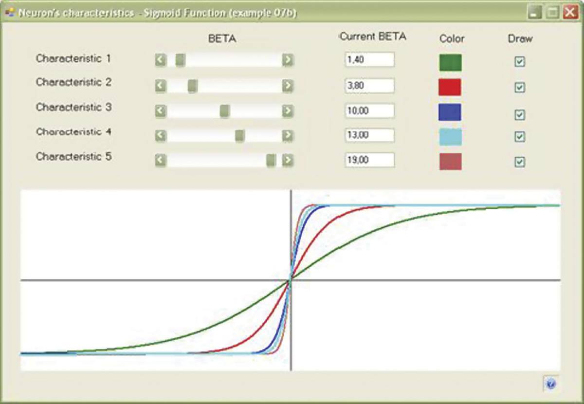
We could find many uses for the transfer functions of neurons. The most popular is the logistic or sigmoid curve. A sigmoid has several advantages: (1) it provides a smooth transition between the 0 and 1 values; (2) it has smooth derivatives that can be calculated easily; (3) it has one parameter (usually called beta) whose value permits a user to choose the shape of the curve freely from very flat (almost linear) to very steep (transition from 0 to 1).

The Example 07b program will allow you to understand transition thoroughly. By building the nonlinear transition function of a neuron, the possibility of moving the “switch” point between the values of 0 and 1 with the use of BIAS is taken into account, but you may also choose the steepness of the curve and general degree of the nonlinear behavior of the neuron (Figure 7.3).

The logistic curve whose properties may be explored with Example 07b has many applications in natural sciences. Every development, whether it involves a start-up company or new technology, follows the logistic curve. At the beginning, growth is small and progress is slow. As experience and resources are gathered, development starts to accelerate and the curve rises more steeply. At the point of success (the steepest section of the ascending), the curve begins to bend toward the horizontal. The bend is almost unnoticeable but growth eventually stops—a state known as satiation. The end of each development involves stagnation (not visible on the logistic curve) and inevitable fall.

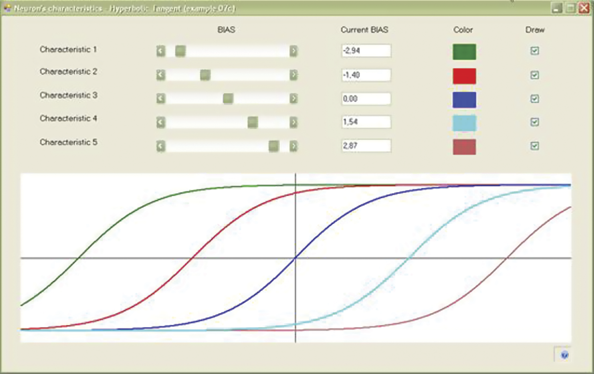
A variation of a sigmoid for bipolar signals (symmetrically arranged between –1 and +1) is a hyperbolic tangent (Figure 7.4). The best option is to examine it in the Example 07c program. After you understand the characteristics of nonlinear neurons, you are ready to build a network from them and start to teach it.

7.4 Functioning of Multilayer Network Constructed of Nonlinear Elements

Multilayer networks constructed from nonlinear elements are currently the basic tools for practical applications and many commercial and public domain programs are available to suit many needs. We will focus on two simple programs intended to demonstrate the functioning of a multilayer network (Example 08a) and a method for teaching such a network (Example 08b).

If you analyze the relevant sections carefully and conduct the experiments by using he programs, you will understand the uses and benefits of backpropagation because it serves a critical function in neural networks and is used universally. After you understand backpropagation, most network issues will be easy for you to recognize and correct in any area of practice.

Program Example 08a shows the functioning of complex network built of only four neurons (Figure 7.5) that form three layers: (1) input that cannot be taught (at top of screen); (2) output where the signals are copied, assessed, and taught (at bottom of screen); and (3) the vital hidden layer shown in the center of the screen. Neurons and signals in the network will be assigned two numbers: the number of the layer and the number of the neuron (or signal) in a layer.

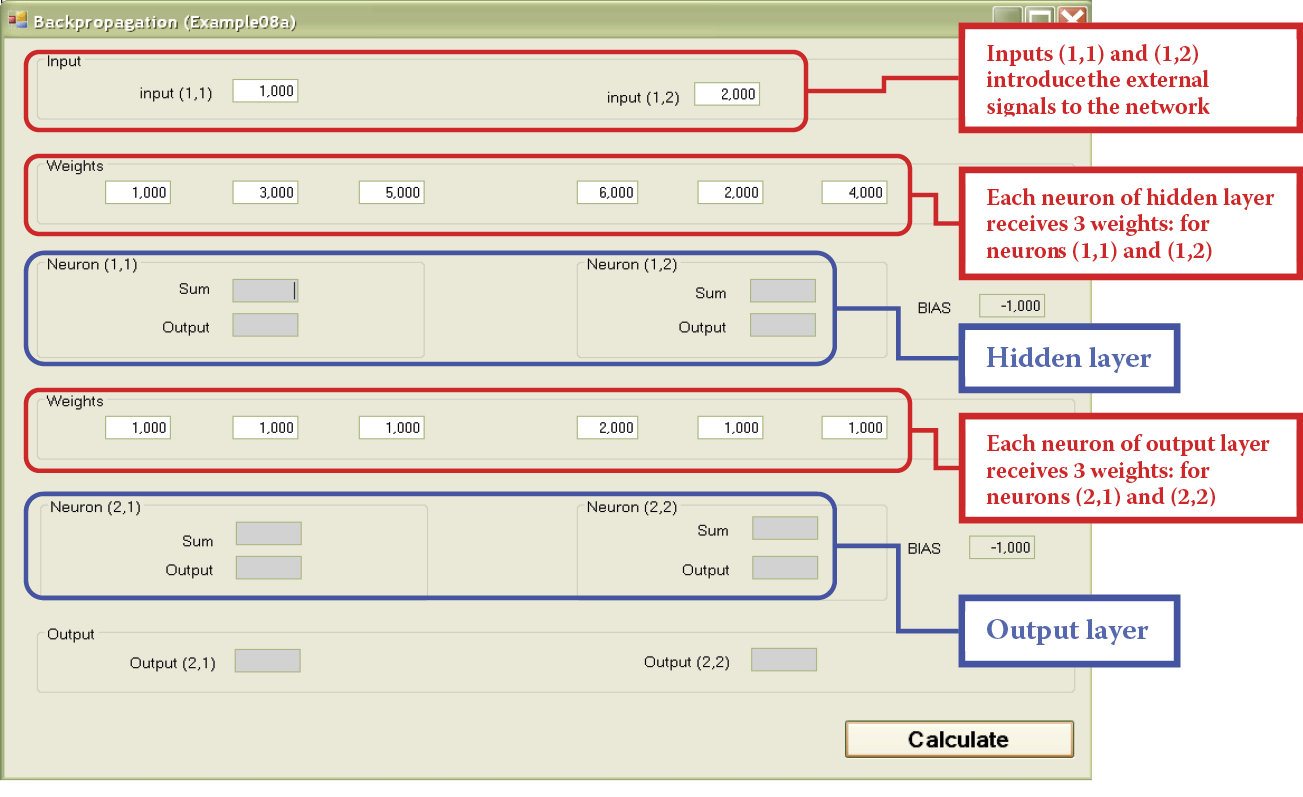
Upon opening, the program asks you to give it the weight coefficients for all neurons in the network (Figure 7.5). You should input 12 coefficients. Our system has four neurons (two in the hidden layer and two in the output layer) to be taught and each of them has three inputs (two from the neurons of the previous layer plus one input also needing a weight coefficient and connected with the threshold that generates an artificial constant BIAS signal.

The advantage of this system is clear. In networks consisting of hundreds of neurons and thousands of weight coefficients, a user does not have to enter all the data because the neurons are designed to set them automatically during the teaching process. In the Example 08a program, you have the option of inputting the parameters to allow you to check whether the output results are what you intended. You will be able to shape the input signals to the network freely and observe both input and output signals of the neurons. Of course, the program includes default values. It is best to choose simple whole numbers as weight coefficients and input signals because they allow you to check easily whether the results produced are those you calculated.

After setting the coefficients, you must determine the values of both input signals (Figure 7.5). The program is now ready to work. Figure 7.6 depicts the beginning of the demonstration.

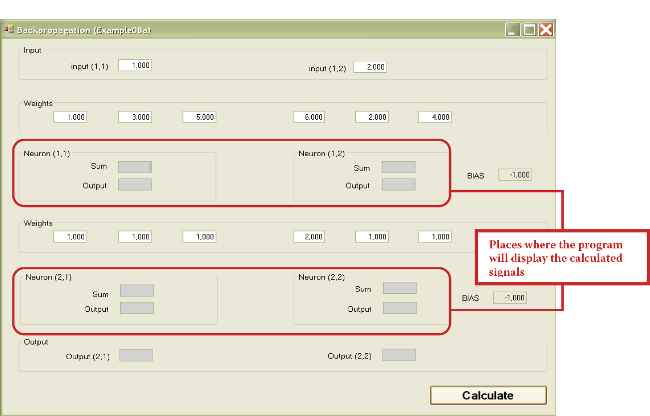
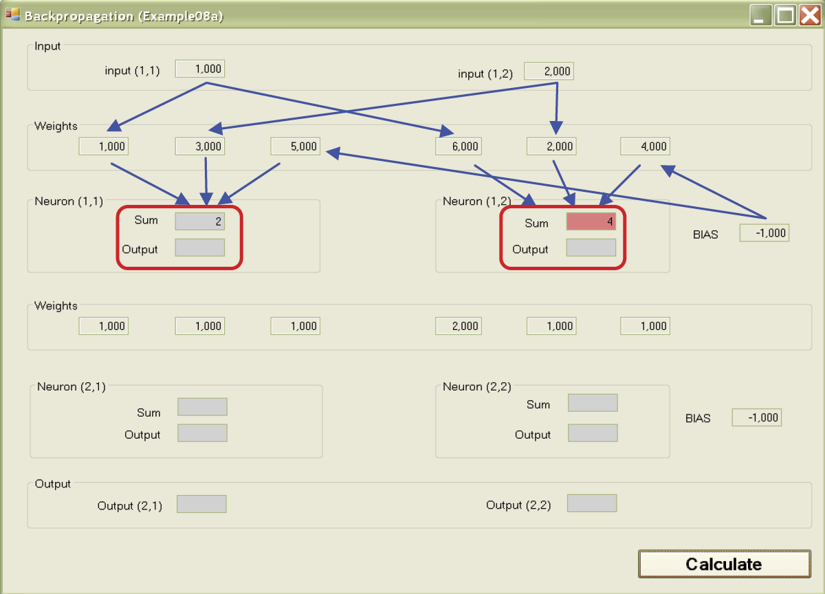
If you click the Calculate button, you will start the simulation process of sending and processing the signals in a modeled network. In each following layer the calculations are made and displayed (against a red background) as the sums of the values of signals multiplied by the correct weights of input signals (along with BIAS component).

Next, the calculated values of the output signals (answers) of particular neurons will be shown (also against a red background) after the added input signals passed through the transfer function. The paths of the signals are shown as arrows on Figure 7.7. The answers of neurons of the lower layer become the inputs for the neurons of the higher layer and the process repeats itself (Figure 7.8).

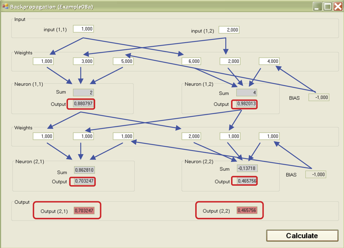
If you press the Calculate button, you can observe the movements of the signals from the input to the output of the analyzed network model. You can change the values of the inputs and observe the outputs as many times as required to ensure that you understand the functioning of the network. We suggest you spend some time reviewing the analysis and the calculations. You can verify results on a calculator to be sure the numbers match those expected. This is the only way you can understand precisely how these networks function.

7.5 Teaching Multilayer Networks

When a multilayer network utilizing your selected weight values and signals holds no more secrets for you, you may want to experiment with it as a learning entity. The Example 08b program is designed for teaching these networks.

After launching this program, you must set the values of two coefficients that determine the course of the teaching process. The first specifies the size of the corrections introduced after finding incoming mistakes and also marks the speed of learning. The larger the coefficient value, the stronger and faster will be the changes in the weights of neurons and detection of errors. This coefficient is called learning rate in the literature. For our purposes, it is called the simple learning coefficient. It must be chosen very carefully because values that are too large or too small will impact the course of learning dramatically.

Fortunately, you do not have to wonder about the coefficient value; the program will suggest an appropriate value. As an exercise, you may want to change the value and observe the effects.

The second coefficient defines the degree of conservatism of learning. The literature defines this quality as momentum—a physical parameter. The larger the value of the momentum coefficient, the more stable and safe is the teaching process. An excessive value may cause difficulties in finding the optimum values of weight coefficients for all neurons in a network. Again, the program uses the correct value based on research but you are free to try other values.

We can now click the Intro button to confirm both values (Figure 7.9). After setting the coefficients as defaults or choosing others, a window displaying neurons, values of signals, weight coefficients, and errors will appear. As an additional aid, the program introduces an additional element that simplifies activities in the form of subtitles at the top of the screen. The simplification is helpful because the tasks of this teaching program are more complex than those of the previous one.

7.6 Observations during Teaching

The task of the modeled network is to identify the input signals correctly. Ideal identification should display Signal 1 in the initial layer of the neuron assigned for a given class (left or right). The second neuron should of course give at the same time a value of 0. To assess the accuracy of network functioning, we can set some less strict conditions. It is sufficient if the error of any output is not greater than 0.5§ because then the classification of the input signal of the network does not differ from the classification given by the teacher.

The notion of error measured as divergence between the real values of input signals and the values given by the teacher as models is not the same as the assessment of the correctness of solutions generated by the network because this assessment involves the general behavior of the network and not the values of single signals. We can often ignore small deviations as long as the network generates correct answers.

Teaching with backpropagation is not likely to be as tolerant as earlier methods as you will see in working with the programs. If an output should have been 1 and the neuron set it at 0.99, backpropagation considers the result an error. However, such perfectionism is an advantage in this situation. Perfect values determined by a teacher enable a network to operate more efficiently.

A school analogy comes to mind here. The concepts learned in geometry do not appear of practical value because we seldom encounter ideal geometric situations in real life. However, an understanding of basic geometry helps us solve practical tasks like determining the amount of fencing required for a building site. Likewise, some knowledge of physics and biology will help you understand the operations of neural networks and apply them as tools in various areas like medicine, economics, and environmental studies.

During teaching, your role will be limited to observation. You simply have to press buttons and review the results on the screen. The program generates the initial values of weights and input signals for identification. Some data such as initial weights and input signals are chosen at random but the models of correct identifications used to teach the network are not random. It may be of help to examine the way the program functions but the network will operate automatically and classify the signals correctly.

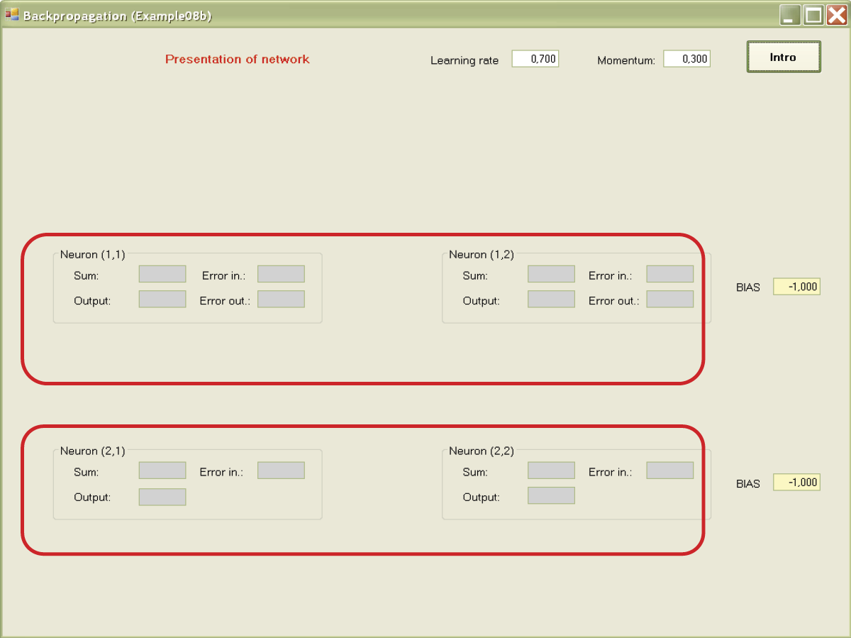
At the beginning the program shows only the structure of the network. Note the subtitles in red at the top of the screen (Figure 7.10). Notice that the sources of BIAS pseudo signals are marked on a yellow background so that they are not mistaken for the sources and values of the signals taking part in teaching.

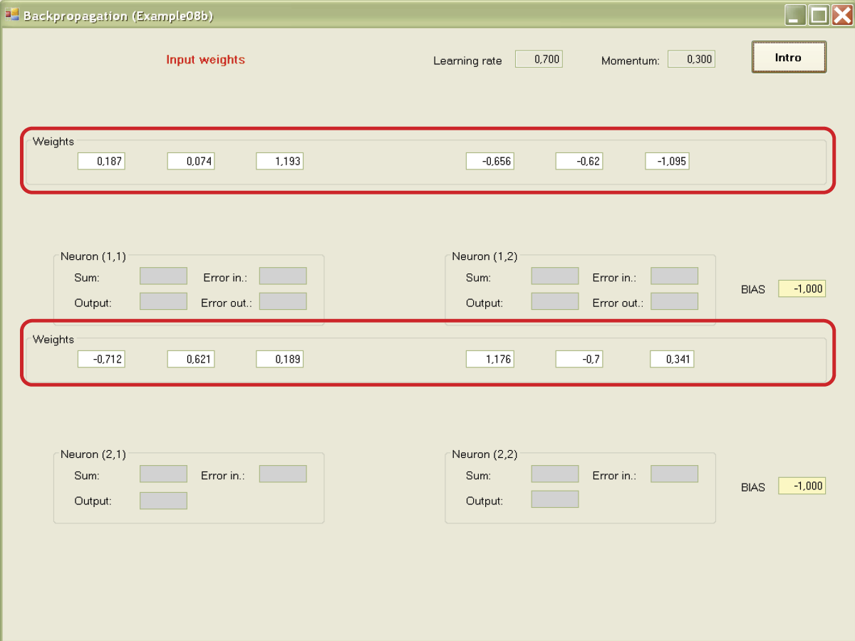
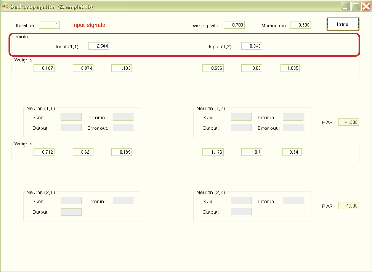
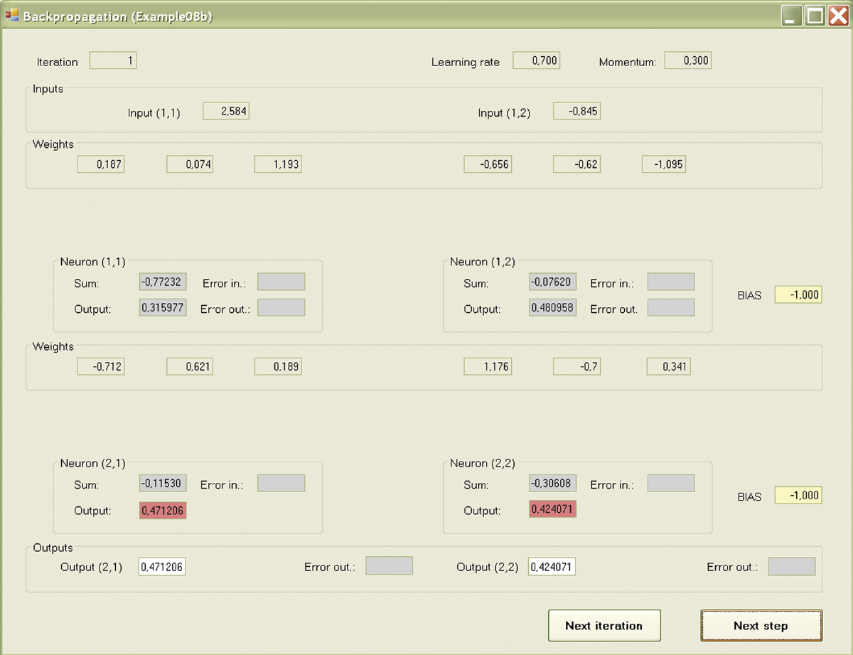
A second press of the Intro button will show you the values of weight coefficients chosen at random at the beginning for all inputs of all the neurons (Figure 7.11). Another click of the button will reveal the values of input signals of neurons [(1,1) and (1,2); Figure 7.12]. Teaching begins at this moment. Your role is limited to pressing the Next button as required to start and conduct a simulation of the network model (Figure 7.13).

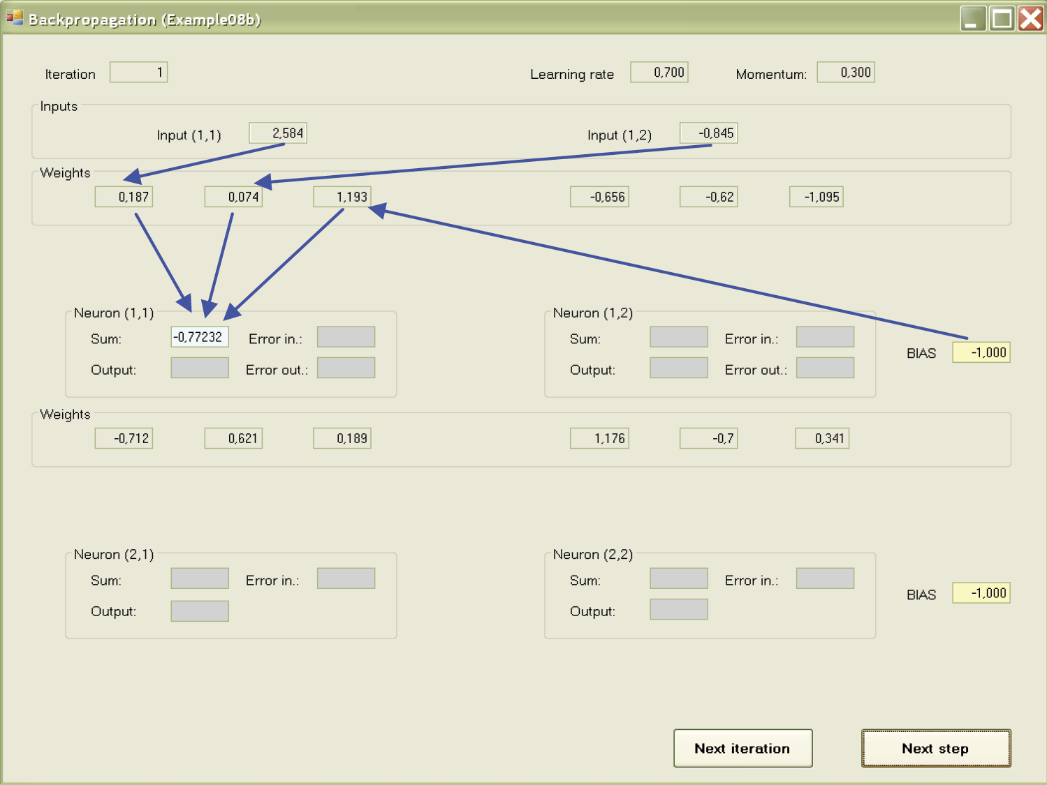
First, the signals calculated to send signals from input to output will be shown for certain neurons. This process is forward propagation. Input signals are recalculated by the neurons on the output signals and the process is conducted in sequence on all layers from input to output. This phase may be observed in the Example 08a program.

Example 08b allows observation of the course of the process with the same precision. First the sums of values multiplied by the correct weights of input signals along with the BIAS component are calculated and the calculated values of the output signals (answers) of particular neurons are shown on a red background. The answers were formed after the sums of input signals were sent through a transfer function with sigmoid characteristics.

The answers (outputs) of neurons of the lower layer also form the inputs of the upper layer. Pressing the Next step button will allow you to observe the movements of signals from the input through output neurons of the model. The target view after several steps is shown in Figure 7.14.

7.7 Reviewing Teaching Results

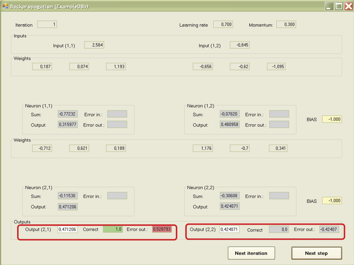
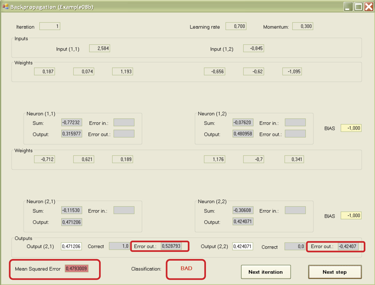
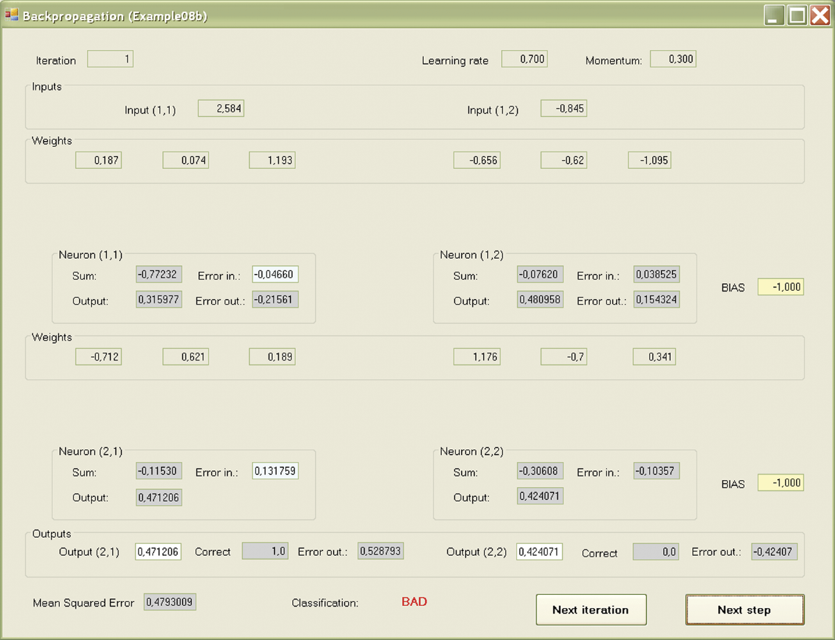
After the signals are fixed on both outputs of the network, “the moment of truth” arrives. The subtitles at the bottom show you the given signals (models of correct answers) for both outputs of the network (Figure 7.15). The errors are marked on the outputs of the network and the mean squared error of both outputs is shown (Figure 7.16).

At the beginning of teaching, network performance may be unsatisfactory. It will improve as the network starts to learn. First the error values are marked for the output neurons of the network. Then the errors are recalculated into corresponding values on the inputs of neurons (that is why we need the differentiable transfer function of a neuron). The errors transferred to the input are marked in Figure 7.17.

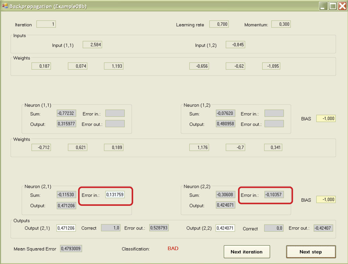
We have now reached the most important stage—propagation of errors to the lower (hidden) layer. The right correct values of respective neurons are shown first as outputs and then by inputs (Figure 7.18). When all error values for all neurons are marked, the next step of the program leads them to setting new (corrected) values of weight coefficients for the entire network. New coefficients appear below the previous ones. A user can review them and determine how far and in which direction teaching changed the parameters of the network (Figure 7.19).

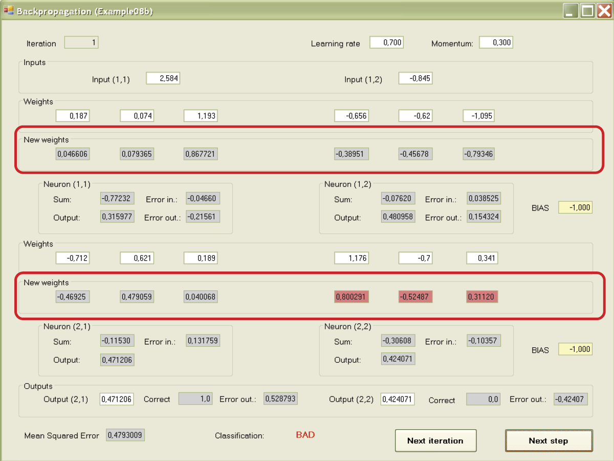
At this point in the program, the screen displays input signals, output signals, errors, and old and new weight values. Analyze the results carefully. The better your understanding of the process, the more chances you have for successful applications of neural networks.

Further experiments with the program can be continued. If you want to review the complete iteration of the teaching process (signal movements, backpropagation of errors, and weight changes), you can press the Next step button. You can also accelerate your review by “jumping” to the moment when the new values of the signals, errors, and weights are marked by using the Next iteration button. This is the most convenient review method. Otherwise, you will have to go through many iterations before the network starts to function correctly.

The review options allow you to observe the teaching process comfortably. You can view the changes of weights and the vital process of projecting the error values in the output layer backward. You will see how the errors of output neurons and errors calculated via backpropagation of hidden layers enable the system to find the needed corrections of values of weight coefficients for all neurons. You will also see the gradual introduction of corrections during teaching. The final result is shown in Figure 7.20.

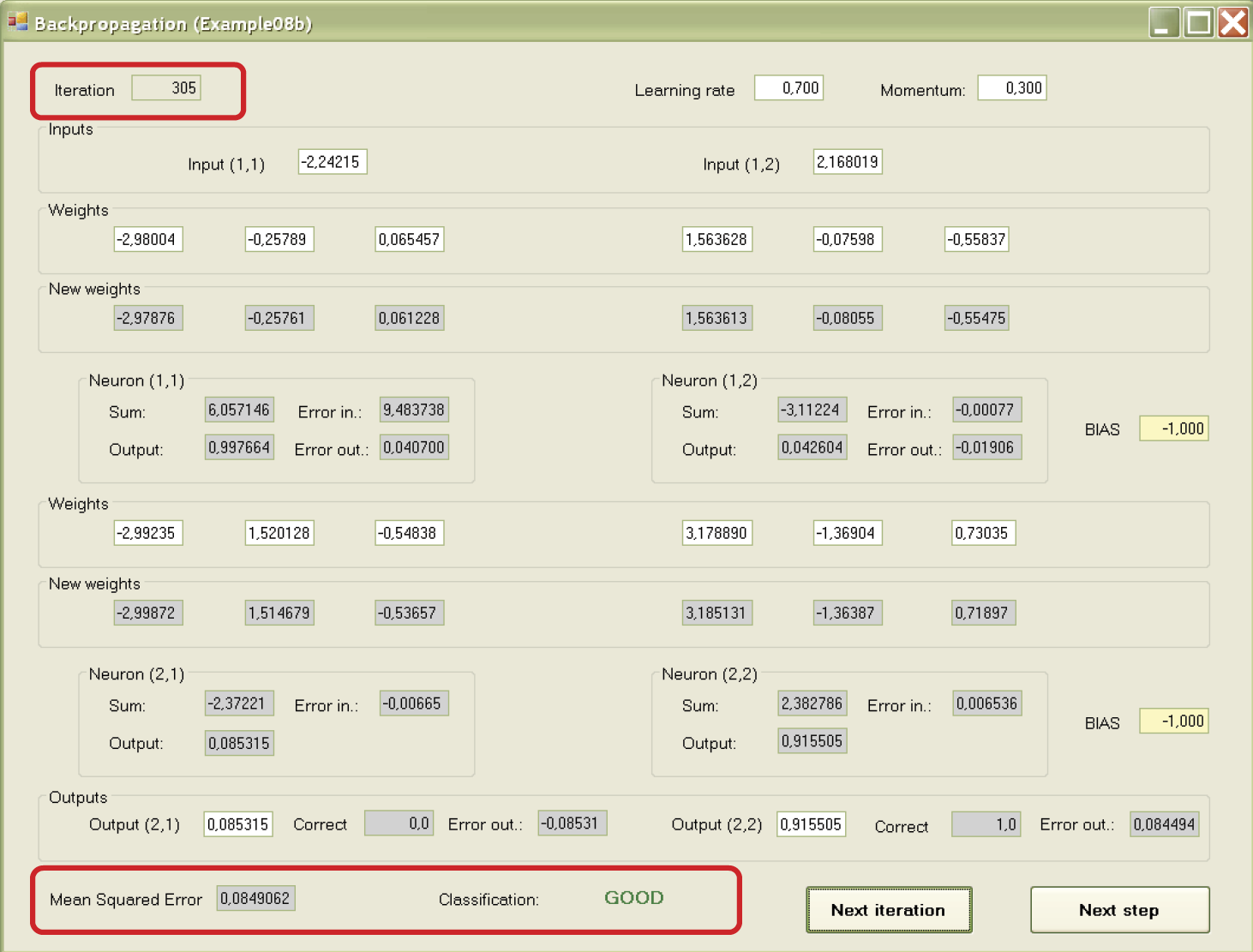
Working with the Example 08b program required some effort because of its complexity. Observing the changing values and processes provided you a tool for understanding backpropagation—one of the most important methods of teaching modern neural networks.

Questions and Self-Study Tasks

1. Why is backpropagation so named? What does it transmit backward?

2. What is BIAS and what does it do? How is the BIAS parameter taught?

3. Why are two values (sum and output) displayed in each neuron during program work? How are they connected?

4. What influences do learning rate and momentum exert on the process of network teaching? Revise your theoretical knowledge and try to explain the influences of these parameters observed during program experiments.

5. What does the transmittal of errors from the output of a neuron (where it is marked) to its input (where it is applied for weight modification) mean?

6. Which neurons of the hidden layer will be most heavily loaded with an error made by a given neuron of the output layer? On what does this effect depend?

7. Is it possible for the neurons of an output layer to show errors if a neuron of the hidden layer has a zero error assigned by the backpropagation algorithm and does not change its weight coefficients?

8. How is the mean mark of the network functioning given? Can we assess the functioning of an entire network using a method that does not require analysis of single elements individually?

9. Advanced exercise: Add a module to the program that will show changes of error values of the neurons and entire network as graphs. Is it true that the functioning of an entire network improves if the errors made by single neurons of the network are minimized?

10. Advanced exercise: Try to expand the programs described in this chapter by using more input and output signals and more neurons arranged in more than one hidden layer.

11. Advanced exercise: Using a network that uses large numbers of inputs, try to observe the phenomenon of “throwing out” unnecessary information in the course of learning. To do so, assign unnecessary information (that has no connection with the required response of the network) to one of additional inputs. The other inputs should receive all data required to solve the required task. After a short period of learning, the weights of all connections leading to “parasitic” inputs to hidden neurons will take values near zero and the idle input will be almost eliminated.

12. Advanced exercise: The program described in this chapter demonstrated the functioning of networks displaying in all places the values of appropriate parameters and signals. This presentation made it possible to check (e.g., with the use of a calculator) what a network does and how it works. However, the program was not very helpful for observing the courses and qualities of the processes. Design and produce a version of the program that will present all values in an easy-to-interpret graphic form.

---