
Chapter 11
Recurrent Networks
11.1 Description of Recurrent Neural Network
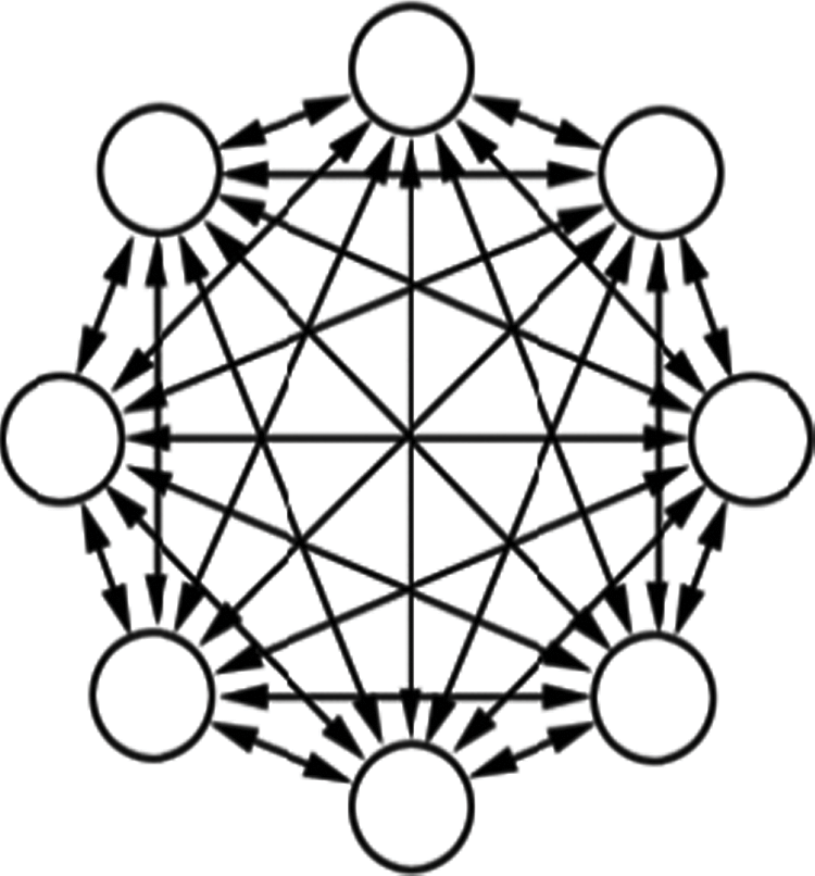
Based on examples described in earlier chapters, you know that a neural network is explained as a single-layer or multilayer, linear or nonlinear system taught by an algorithm or discovering knowledge on its own. The neural networks discussed to this point are almost free to choose their learning parameters. We say almost because we have not covered recurrent networks yet. These networks include feedback mechanisms that recycle signals from neurons in the input layer to neurons of previously hidden layers (Figure 11.1). Feedback is a relevant and significant innovation. As you will see, a network with feedback has more upgradable possibilities and computing capabilities than a classical network restricted to one-way signals from input to output.
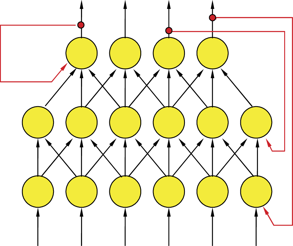
Example of recurrent network structure. Feedback connections are distinguished by exterior arrows in red color.
Networks with feedbacks show phenomena and processes not revealed by one-way networks. After stimulation, a network with feedback can generate thorough sequences of signals and phenomena as outputs (results of signal processing in n iteration) and return to the inputs of neurons to produce new signals, usually in n + 1 iteration. Specific phenomena and processes of recurrent networks arise from complicated signal circulations (e.g., vibrations varying between the rapid rise of alternate extremes), equally rapid suppressions, or chaotic roaming (that looks like undetermined progress).
Recurrent networks with feedbacks are less popular because they are difficult to analyze. Their ability to circulate signals through a network from input to output, then from output to input, and then back to output requires a more complex structure than a simple one-way system. The recurrent neural network responds to every input signal, even short-term types. It proceeds through long sequences of intermediate states before all essential signals are established.
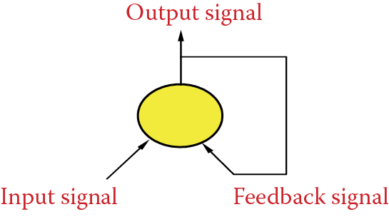
We will use a simple example to illustrate how a recurrent device works. Imagine a linear network consisting of only one neuron. It has two signals: the first is an input signal and the second is an output signal that becomes the second input. Thus we created feedback (Figure 11.2). It was easy, wasn’t it?
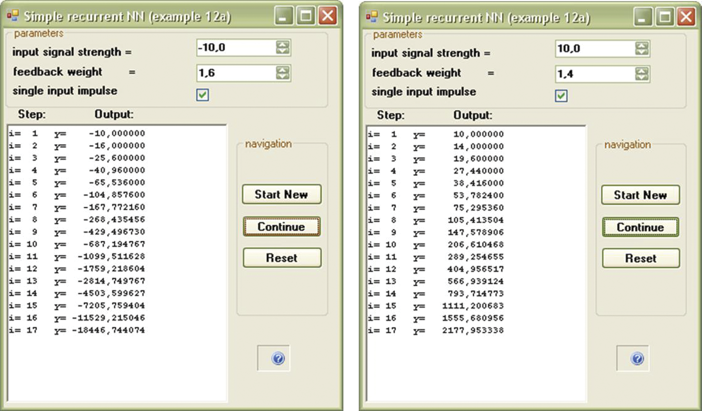
We now check how this network works. We can use Example 12a in Figure 11.3 to determine its parameters. Weight factor (feedback weight) determined by a feedback signal will enter the neuron along with the input signal (input signal strength) that runs the network. You can decide (by activating or not activating single_input_impuls) whether the input signal will enter continuously or temporarily (only once at the beginning of simulation). This program will compute signals going around a network, step by step, demonstrating network behavior. You will quickly notice a few characteristics:
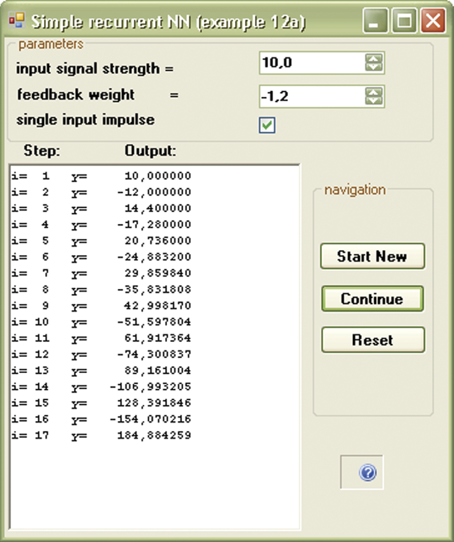
- The described network displays combined dynamic forms: after entering a single (pulse) signal at the input, the output sustains a long-lasting process, during which the output signal changes many times before it can reach the state of equilibrium (Figure 11.3).
- Equilibrium in this simple network may be achieved (without output signal that continues throughout the simulation) only if a constant product of a certain output after multiplying by weight of a proper input yields an output signal precisely equal to the feedback signal needed to create an output signal; signals at both neuron inputs will balance themselves out.
- An output signal that complies with this condition is called an attractor. We will soon explain this term.
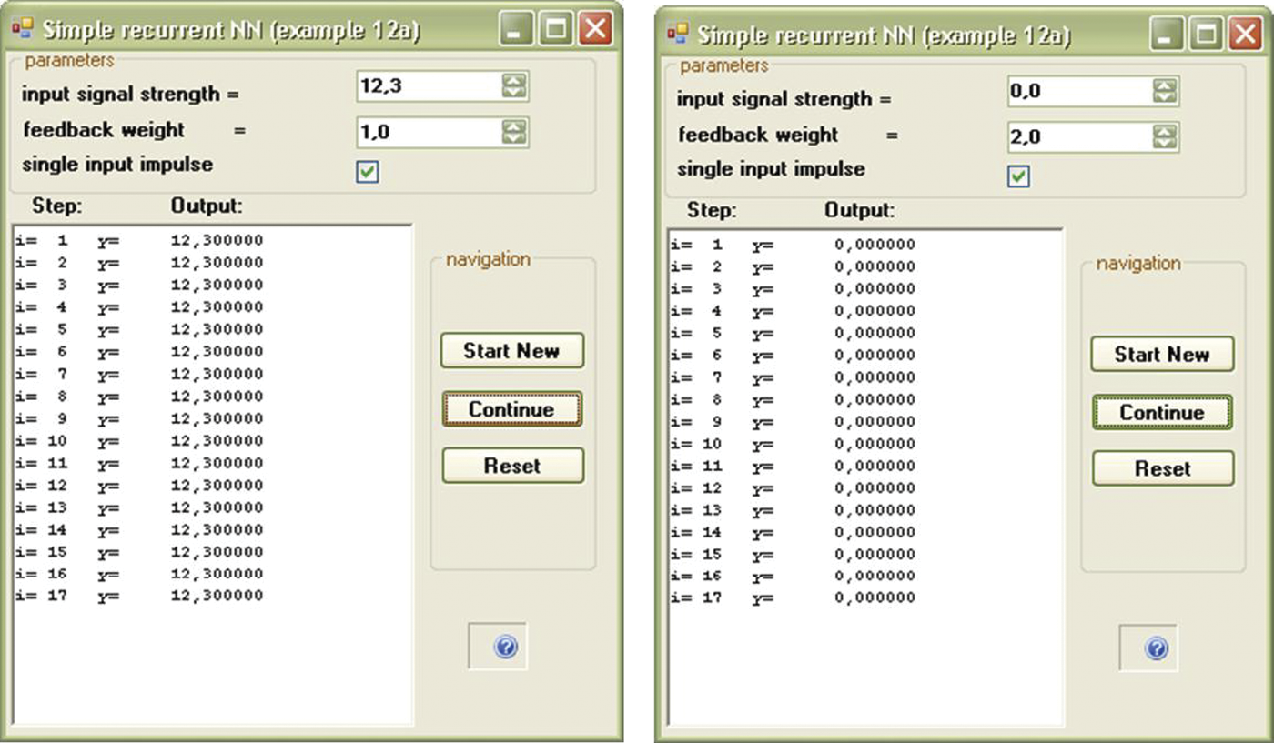
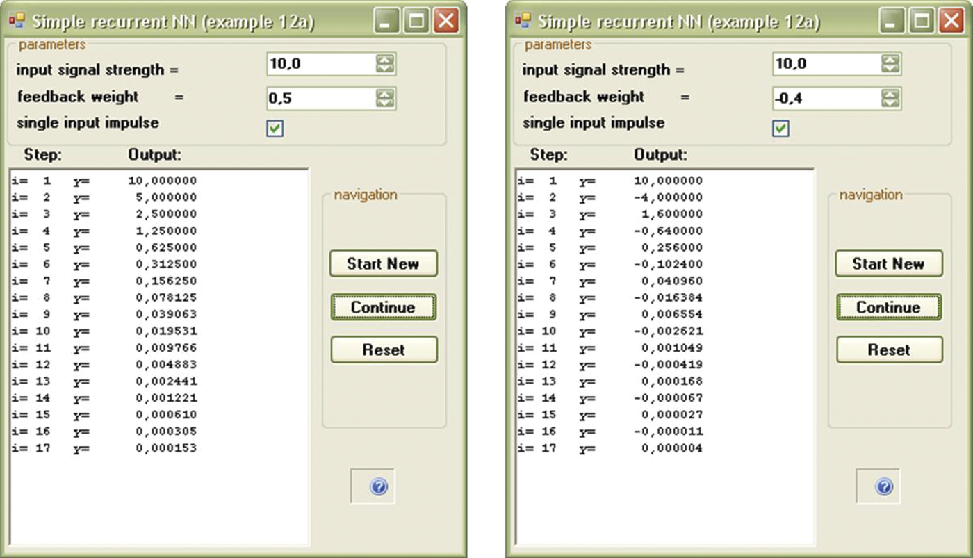
- Attractor location depends on network parameters. For a network with a weight factor of feedback value of 1, every point is an attractor. For any other network, we can achieve equilibrium only when the value of the output signal is 0 (Figure 11.4). This feature is distinctive for this simple linear network. Nonlinear networks obviously involve more attractors and we will make use of them.
- If the value of a synaptic weight factor in a feedback circuit is positive (positive feedback), the system displays an aperiodic (non-oscillating) characteristic (Figure 11.5). It is worth noting that this process may proceed through positive values (left side) of signals or negative (right side) values. As time passes, positive values become more positive and negative values become more negative. No processes allow signals to change from positive to negative or vice versa.
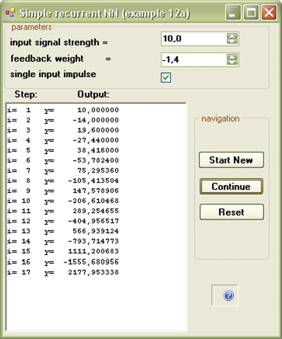
- If the value of a synaptic weight factor in a feedback circuit is negative (negative feedback), the system displays a periodic (oscillating) characteristic (Figure 11.6).
- In systems with negative feedback, oscillating character depends on network parameters. If vibrations increase rapidly, a network may toggle between large negative values and even larger positive values, followed by larger negative values and so on. This is catastrophic. The network behavior closely resembles that of human brain suffering from epilepsy or a space rocket that loses stability during take-off and crashes. However, vibrations sometimes lead to zero values, the network is stabilized, and work is handled correctly.
- While observing behavior of systems with feedbacks, you will see that even small differences in parameters values will cause effects that may be extreme. Systems without feedback do not produce such differences. This somewhat extreme reaction is a distinctive feature of recurrent systems.
- We now analyze the above phenomena quantitatively. After few simulations, if the absolute value of a weight factor in feedback exceeds a certain established value (stabilization point), absolute values of signals continuously increase in both systems with negative feedback, and systems with positive feedback (Figure 11.5 and Figure 11.6). This phenomenon is known as unstable behavior.
- However, if the absolute value of weight factor in feedback is smaller than the established value, a circuit with either positive or negative feedback will attempt to reach equilibrium (Figure 11.7).
An input signal could be also given for the duration of simulation by unmarking the single_input_impulse checkbox (Figure 11.8). The state of equilibrium may be achieved, but the value of the output signal (the network is stabilizing for this signal) is different and depends on the input signal value.
Two ways of achieving state of equilibrium in a linear network: zero signals (left) or single feedback amplification without simultaneous input signal (right).
Stable progress of system with feedback after decreasing value of weight factor well below stabilization point.

11.2 Features of Networks with Feedback
Let us summarize and draw conclusions of some researchers that will be useful when we follow the next steps. Processing of input signals in a network with feedback can display two different variabilities. First, if the value of a weight factor in feedback is positive, the signal changes aperiodically (in one way). Second, when value of a weight factor in the feedback is negative (regulation), oscillations occur in a network by which the output signal alternates between lower and higher values.
If a neuron is nonlinear, the system may behave in a third way involving roaming chaotic signals (“butterfly effect,” strange attractors, fractals, Mandelbrot’s sets, etc.). We will not cover this type of operation in this chapter but much information is available on the web.
Along with dividing network behavior into aperiodic and periodic sections, networks with feedback display stable behaviors (signals with value restraints that usually converge into a certain final value after a few iterations) and unstable behaviors in which absolute values of successive output signals increase in size and finally exceed acceptable values. During simulation, these behaviors give rise to mathematical errors like floating point overflow. In electronic or mechanical systems, components may burn or explode. All these behaviors also occur in real neural networks.
Positive feedback creates a progressive effect. It is an amplification of positive values of signals in a system as shown on the left side of Figure 11.5. An inverse effect is similar to a human’s negative attitude toward some experience and is depicted on the right side of Figure 11.5. If a closed circuit of positive feedback is not disconnected, it can produce disturbances. The condition is dangerous in humans. Negative amplification leads to a condition called manic psychosis; excessive amplification of positive values can create an unrealistic state of euphoria. Non-stability phenomena also occur in human nervous systems. One result is a grave illness called epilepsy. It is characterized by brief disturbances of electrical activity in the brain that cause rapid involuntary muscular contractions and convulsions. It is easy to see how incorrect functioning of artificial neurons and the consequences resemble nervous system malfunctions in humans.
We suggest you use your computer to detect the stabilization limits for a simple system with feedback. Try to discover which factors cause stable or unstable behavior. You can then use the Example 12a program to compare your findings. As you work with Example 12a, you will notice that output signal alterations depend on factor values whereas input signals exert weaker influence both at the start of a program and during operation.
When examining network behavior and considering algorithms, it is important to know whether the absolute value of weight factor for a feedback signal is more or less than 1. For factors less than 1, you have a stable process—aperiodic for positive values and oscillating for negative values. The process is always unstable for factors greater than 1. When a value of factor is exactly 1 and feedback is positive, all input signals will be network attractors. Negative feedback produces continuous (not fluctuating) oscillations. We call this state the stabilization limit.
In more complex networks, stabilization conditions are more complicated and calculation of stabilization limits requires advanced mathematical methods such as Hurwitz‘s determinants, Nyquist‘s diagram, Lyapunow‘s theorem, and others. The theory of neural networks with feedback in complex dynamic systems has been an active research area for all kind of theorists for many years.
11.3 Benefits of Associative Memory
The operation of a network consisting of a single neuron is simple and easy to predict, so the opportunities to observe interesting practical applications are limited. That is why the Example 12a program does not yield practical results. Large networks of dozens of nonlinear neurons and feedback capability display complex and interesting behaviors that serve as bases for practical applications. However, large networks with many neurons that transfer output signals to each other via feedback are also open to more operational issues and unstable behaviors than single neuron systems. In a complex network, states of equilibrium may be achieved by different values of output signals, but it is possible to select certain joint structures and certain network parameters to ensure that the states of equilibrium will be equal to the solutions to certain problems.
This is a requirement for most nontrivial network applications. For instance, in some networks, the state of equilibrium is the solution of an optimization problem after a search for the most beneficial decision that will ensure the highest gain or smallest loss by taking restraints into account. These networks are capable of solving the well-known traveling salesman problem used as a training example. They have been used to research optimal distribution of finite resources such as water and select investment portfolios.
That is why in this chapter, we are going to present you another example in which solution of a certain important and useful computer problem could be interpreted as achieving one among many states of equilibrium by network: so-called associative memory. This type of memory the goal of many computer scientists who are tired of current methods that require searching for information in primitive data bases. We will discuss this kind of memory and how it works.
We all know that storing millions of records that include vital information can be accomplished effortlessly with few delays. The task is simple if you understand key words, code words, specific values, and other items that differentiate one record from others. A computer will find any record and allow access. The process is quick and efficient if the base is indexed and constructed appropriately. A Google search is a good example of this process.
Retrieval of data does not look so simple when you do not have key words or other identifying information to focus your search. If you do not know how the desired information is described by the search system, you may receive outputs that are unresponsive or unreliable. You may receive plenty of unnecessary information if you cannot provide specific search data. Excessive information is the lesser of the two evils of retrieval; the other is inadequate information. Narrowing a search to dig out essential data may be described as drudgery.
Usually you need just a scrap of information to find what you want effortlessly. Sometimes a single word, image, picture, conception, idea, or formula will deliver instantly a complete collection of data, references, suggestions, and conclusions. This is similar to the way a fragrance, melody, or sunset can trigger the human brain to deliver memories, feelings, and senses. Based on a bit of information, your brain can respond to a request. Computers do not know how to respond to such triggers yet, but what about neural networks?
Associative memory represents a small segment of a discipline called cognitive science that has attracted increased attention recently, especially among philosophers, pedagogues, and psychologists. Many specialists are passionately fond of this subject, especially physicists, who normally work with theoretical descriptions of simple physical systems of elementary particle or specialize in describing systems composed of many interacting particles (statistical thermodynamics). If you search a library or the Internet, you will see that a huge number of physicists are conducting research in this area.
Their research focuses on the behaviors of networks when exposed to feedback and other processes that may lead to practical applications. This is how the so-called Boltzmann machines were developed. They utilize thermodynamic phenomena based on algorithms of simulated annealing and Boltzmann’s distribution analogous to the operations of neural networks. Professor Jacek Zurada at the University of Louisville in the U.S. and Professor Leszek Rutkowski of Czestochowa University in Poland specialize in cognitive studies, specifically simulation of neural networks. They have made significant contributions to the field, but the greatest contribution was made by John Hopfield, a US scientist who studied network feedback.
11.4 Construction of Hopfield Network
Hopfield’s networks constitute the most important and most often adapted subclass of recurrent neural networks used in practice and that is why readers should understand them. If we had to classify them, they act as exact opposites of feed-forward networks described in earlier chapters. Networks in which feedbacks are allowed (so-called recurrent networks) can contain a certain number of feedbacks, whereas feedbacks in Hopfield networks are not real (Figure 11.9).
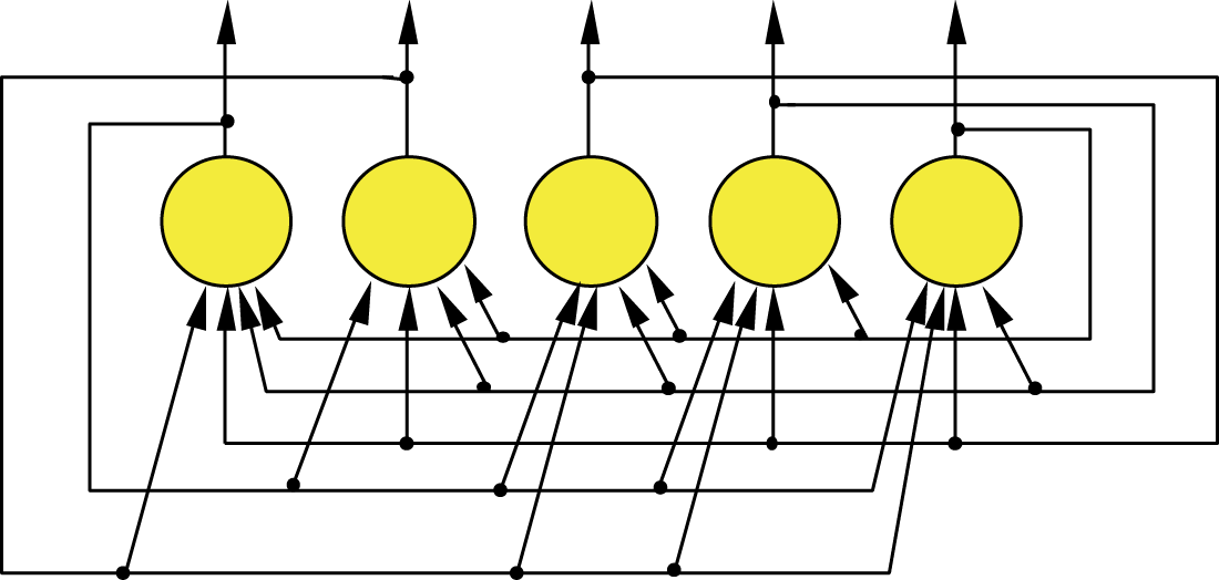
All joints in non-Hopfield networks are feedbacks, all output signals are employed as inputs, and all inputs transport feedback signals to all neurons. In Hopfield’s network, each neuron is connected to all other neurons within entire network, The connections are based on the two-sided feedback rule so a Hopfield network looks and acts like a single-feedback network. Hopfield’s system is an exact opposite of earlier networks that without exception were feed-forward networks—feedback was impossible.
Hopfield networks are important because their processes are always stable. Thus these networks work effectively and users need have no anxiety about failure. The stability of processes in a Hopfield network was achieved by the application of a few simple concepts.
They are easy to design and use as computer programs and also in certain specialized electronic and optoelectronic circuits. The internal structure of the network is based on connecting all the neurons in an everyone-with-everyone fashion. This simple (and costly) principle was used in networks described earlier (e.g., networks taught by the backpropagation method; see Chapter 7) in which connections of neurons from hidden layers and neurons from the output layer were organized this way. Hopfield’s network uses tested models but involves one significant difference. Connected neurons work as both information transmitters and also as information transceivers. They constitute one collective system (Figure 11.10), not separate layers.
Scheme of Hopfield network emphasizing equality of rights of all neurons and symmetry of connections.
Another important characteristic of the Hopfield network is that feedbacks involving one neuron are impossible. An output signal cannot be given directly to its input neuron. This principle is obeyed in Figure 11.9. Notice that it does not rule out a situation in which an output signal from certain neuron influences its own value in the future because it can achieve feedback via other (intercalary) neurons that provide stability (Figure 11.10).
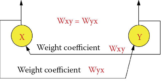
The entered weight factors must be symmetrical. If a connection from neuron X to neuron Y is defined by a certain weight factor W, the weight factor defining the connection from neuron Y to neuron X has the same W value (Figure 11.11). We can fulfill these conditions effortlessly. The first two describe a simple scheme of connections. If you choose Hebb’s method (described in Chapter 9) to teach your network, the final one condition is met automatically.
The simple structure and easy application of Hopfield networks made them highly popular. They are widely employed in various optimization tasks and to generate certain sequences of signals that follow each other in a specific (and modifiable) rotation. These networks made it possible to generate and forward control signals to many types of objects, for example, walking machines that stand on two, four, or six legs (Figure 11.12).
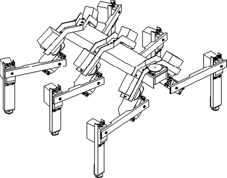
Treading robot. Legs are controlled by periodic signals generated by its “brain” (Hopfield network).
The “brains” that control movements of these machines always includes feedback components that allow the machines to generate their own control signals periodically. Treading machines, regardless of the number of legs, follow a consistent process by which each leg in a specific order is lifted, moved forward, lowered until it contacts a stable surface, and moved back to transport its “body” forward. Each leg also provides support when the driving force is provided by other limbs.
Treading on a rough surface requires all these movements and an additional mechanism that will adjust the machine to accommodate a changing situation such as an uneven surface. Thus, such machines must be able to generate consistent behaviors and adapt to changing situations. A Hopfield network meets these challenges. Intelligent learning and treading robots have been developed for exploring remote planets, cave interiors, and ocean floors, but for now we will use a Hopfield network to construct associative memory.
11.5 Functioning of Neural Network as Associative Memory
The Example12b program contains a Hopfield network model designed to store and reproduce simple images. The whole “flavor” of this memory lies in its ability to reproduce a message (image) on the basis of a strongly distorted or disturbed input signal. The phenomenon is called auto-association* and it allows a Hopfield network to seek incomplete information. Figure 11.13 has been reprinted and reproduced on the Internet (www.cs.pomona.edu and eduai.hacker.lt) many times. It illustrates the efficiency of a Hopfield network in removing interference from input signals and completely recovering data in cases where the inputs consisted only of fragments.
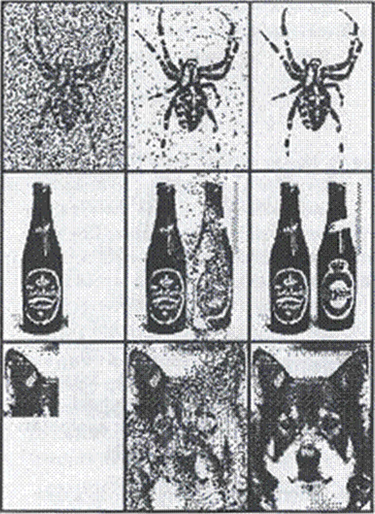
The next three lines of this figure show each input. The middle column shows the transition state when the network searches its memory for the proper pattern. The right section shows the result—reproduction of a complete pattern. Of course, before the network could “remember” the relevant images, they had to be fixed in the learning process. During learning, the network was shown images of a spider, two bottles, and a dog’s head. The network memorized the patterns and prepared to reproduce them. When the network was shown a “noisy” picture of a spider (top row of Figure 11.13), it reconstructed the image of the spider without noise. When shown a picture of one bottle, it remembered the two bottles presented during learning. Finally, showing the dog’s ear to the network was sufficient for it to reconstitute the whole picture.
Figure 11.13 is interesting but does not relate to practical tasks. Despite the whimsical example, auto-associative memory can serve many practical purposes, for example, reproducing a complete silhouette of an aircraft from an incomplete camera image obscured by clouds. This ability is critical for military defense systems that must quickly differentiate friend from enemy. A network employed as an auto-associative memory can provide complete answers based on incomplete information in a database if the user asks questions correctly. If a question posed to such a network does not correspond to preconceived models, the database will not know how to respond.
Auto-associative memory can work effectively with database management programs to ensure that searches will be performed correctly even if a user inputs an imprecise query. The network will be able to provide the missing details. An auto-associative Hopfield network mediates between a user and a database like a wise librarian who knows what book a student wants even if the student has forgotten the author, title, and other details.
Auto-associative networks are useful in other ways, for example, removing noises and distortions from signals when noise levels preclude the use of common methods of signal filtration. The extraordinary effectiveness of Hopfield networks results from their ability to utilize a distorted or incomplete image as a starting point and reproduce the complete image based on stored information.
We can now proceed to practical exercises using the Example12b program. For demonstration purposes, we will illustrate Hopfield network performance using pictures, but remember that such networks can memorize and reproduce any other type of information based on how it is mapped and represented.
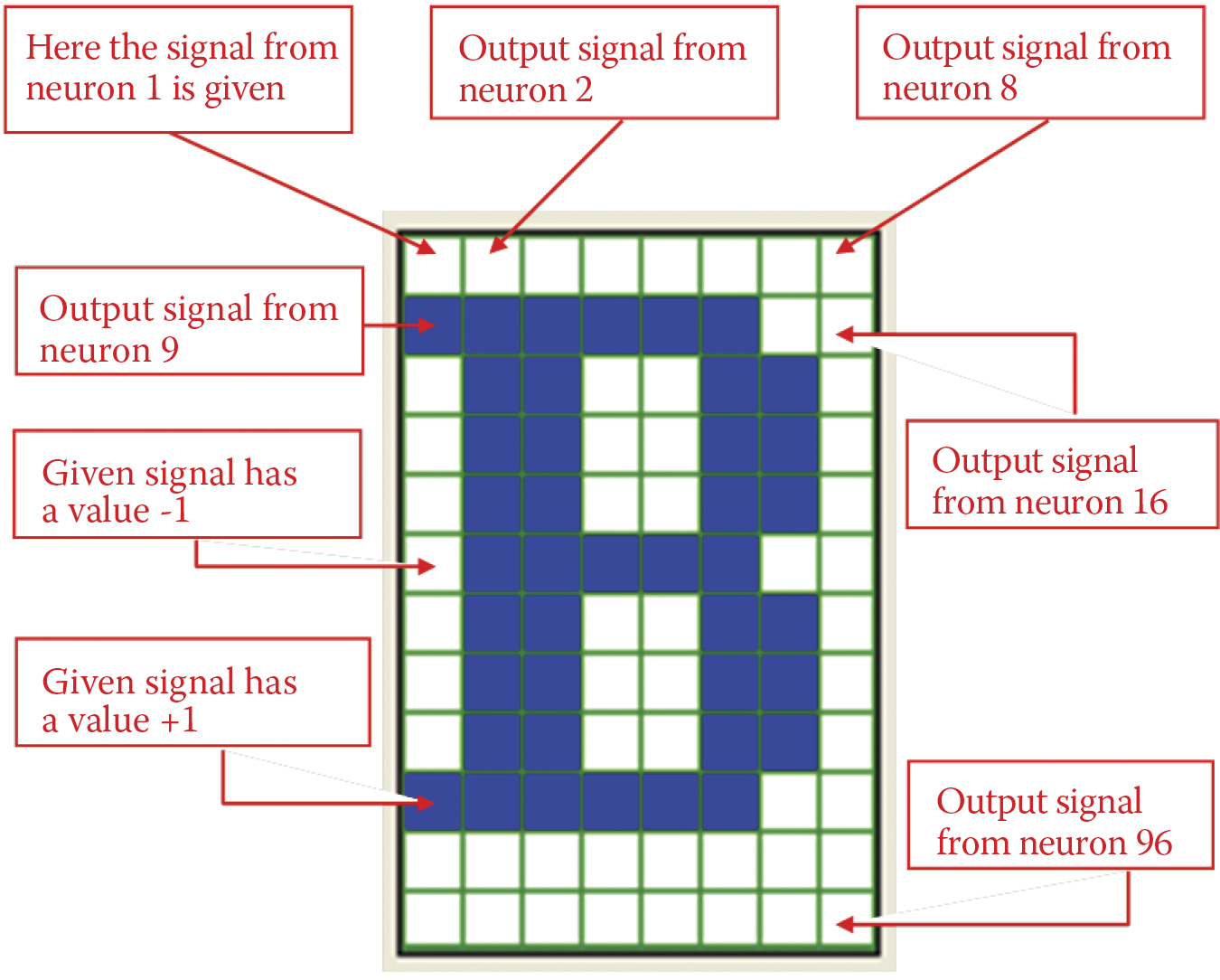
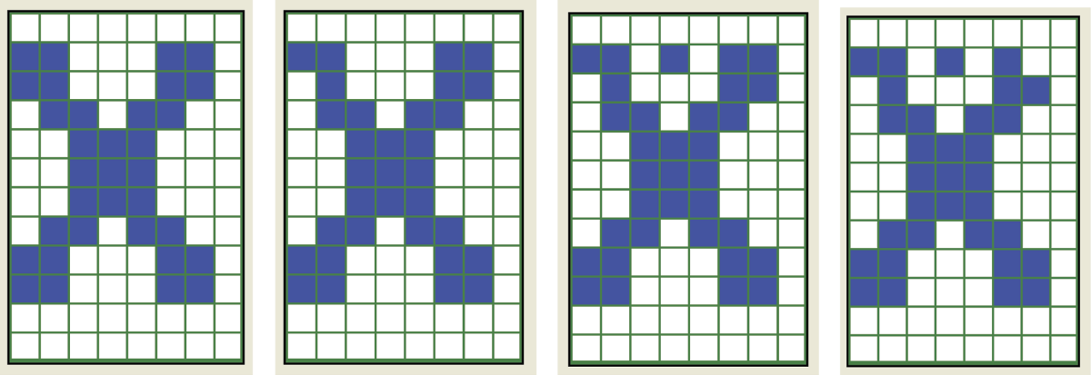
You should understand the relationship between the modeled Hopfield network and the pictures presented by a program. Each neuron of the network is connected with a single point (pixel) of an image. If the output signal of the neuron is +1, the corresponding pixel is black. If the output neuron signal is –1, the corresponding pixel is white. We will not consider other color possibilities because the neurons used to build a Hopfield network are highly nonlinear and can be distinguished only as +1 or –1 and cannot handle other values. The considered network contains 96 neurons that for presentation purposes are arranged as a matrix of 12 rows of 8 items each. Therefore, each specific network state (set of output signals produced by the network) can be seen as a monochrome image of 12 × 8 pixels as shown in Figure 11.14.
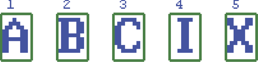
Illustrations for presentation may be chosen arbitrarily, but we limited our choices for creating a set of tasks for the network. We chose images of letters (because they are easy to input via a keyboard) or abstract images produced by the program based on certain mathematical criteria.
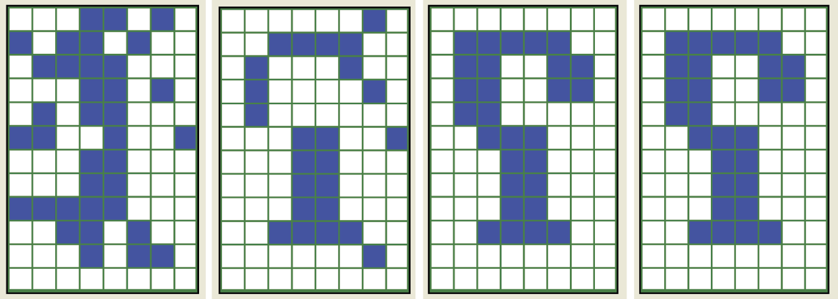
The program will remember a number of images provided by a user or generated automatically and then list them (without user participation) as patterns for later reproduction. Figure 11.15 depicts a set of patterns to be remembered. Of course, a set of patterns memorized by the network may include any other letters or numbers that you can generate on a keyboard, so Figure 11.15 should be considered one of many possible examples.
The process of introducing more patterns to the program will be explained shortly. Initially, we want to focus on what this program does and what the results are. The technical details will follow shortly.
After the introduction of all the patterns, Example12b sets the parameters (weight factors) of all neurons in the network, so that these images become points of equilibrium (attractors) for the network. We will not go into an explanation of the theory of Hopfield network learning because it involves difficult mathematical equations and calculations. After the example program introduces new patterns into the network memory, you simply click the Hebbian learning button.
This automatically launches the learning process, after which the network will be able to recall its stored patterns. The learning of the network is realized by Hebb’s method that was explained earlier. Keep in mind that the values of weights produced by this learning process will reach equilibrium state when its output images appear to match a stored pattern.
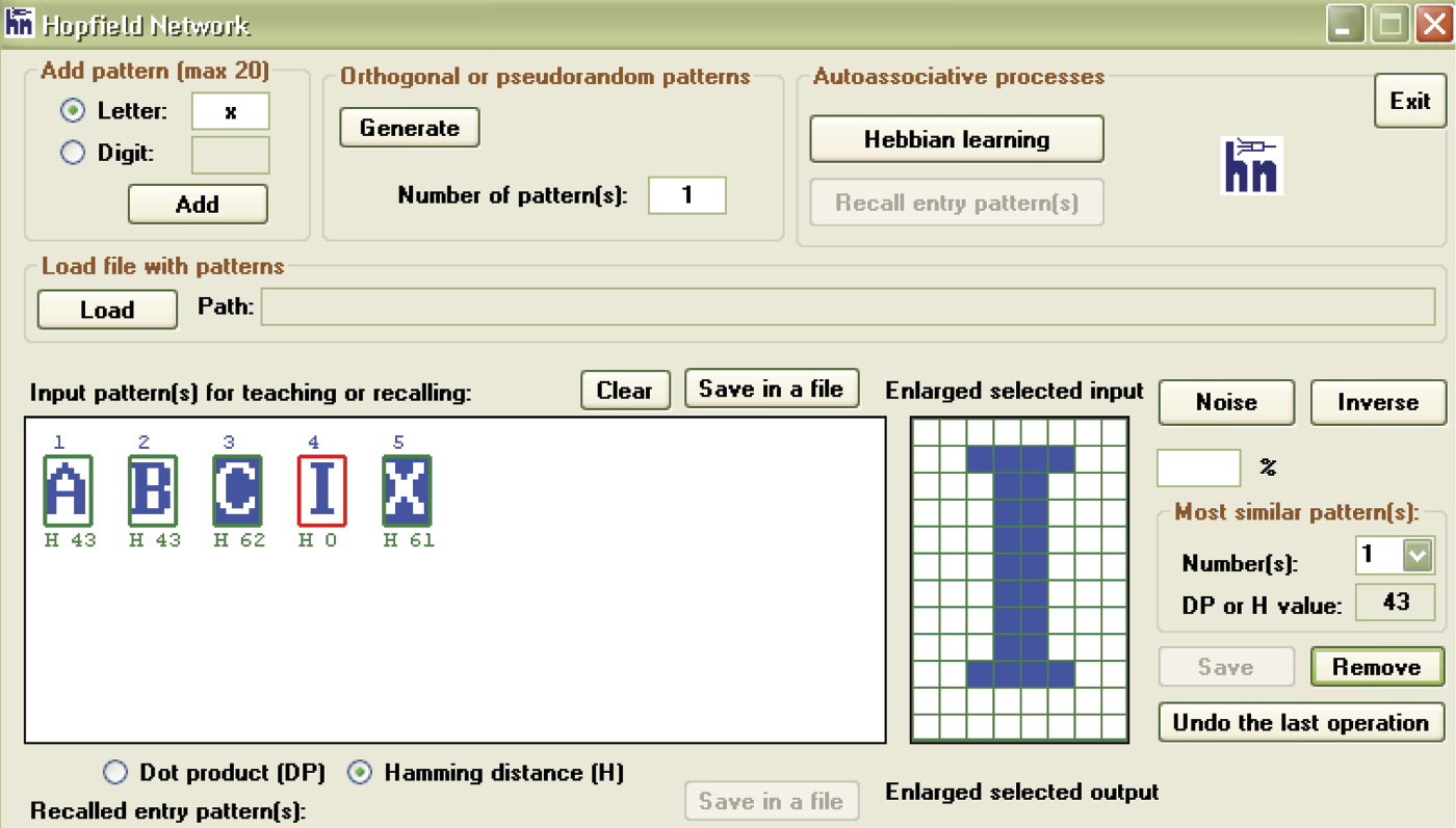
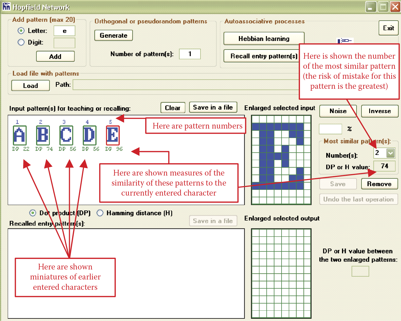
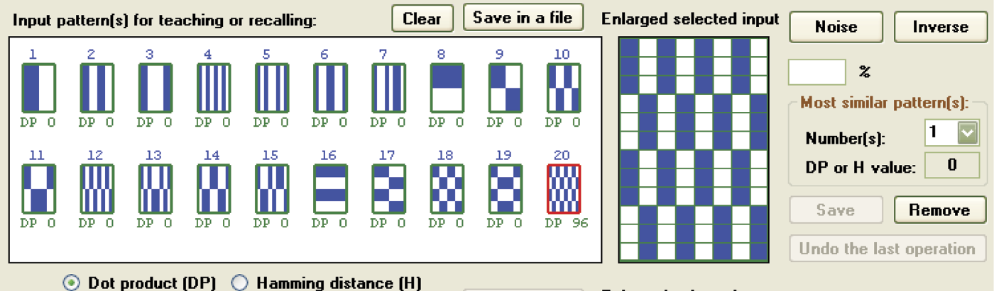
After learning is complete, the network is ready for testing. First point at the pattern for the level of control you want to check. Patterns and their numbers are visible as inputs in the teaching or recalling window and you can choose the one you want the network to remember. Selection of any pattern will cause its enlarged image to appear in the window titled Enlarge selected input. The chosen measure of its similarity to all other models will be visible directly under the miniature images of all the patterns in the Input pattern(s) window (Figure 11.16).
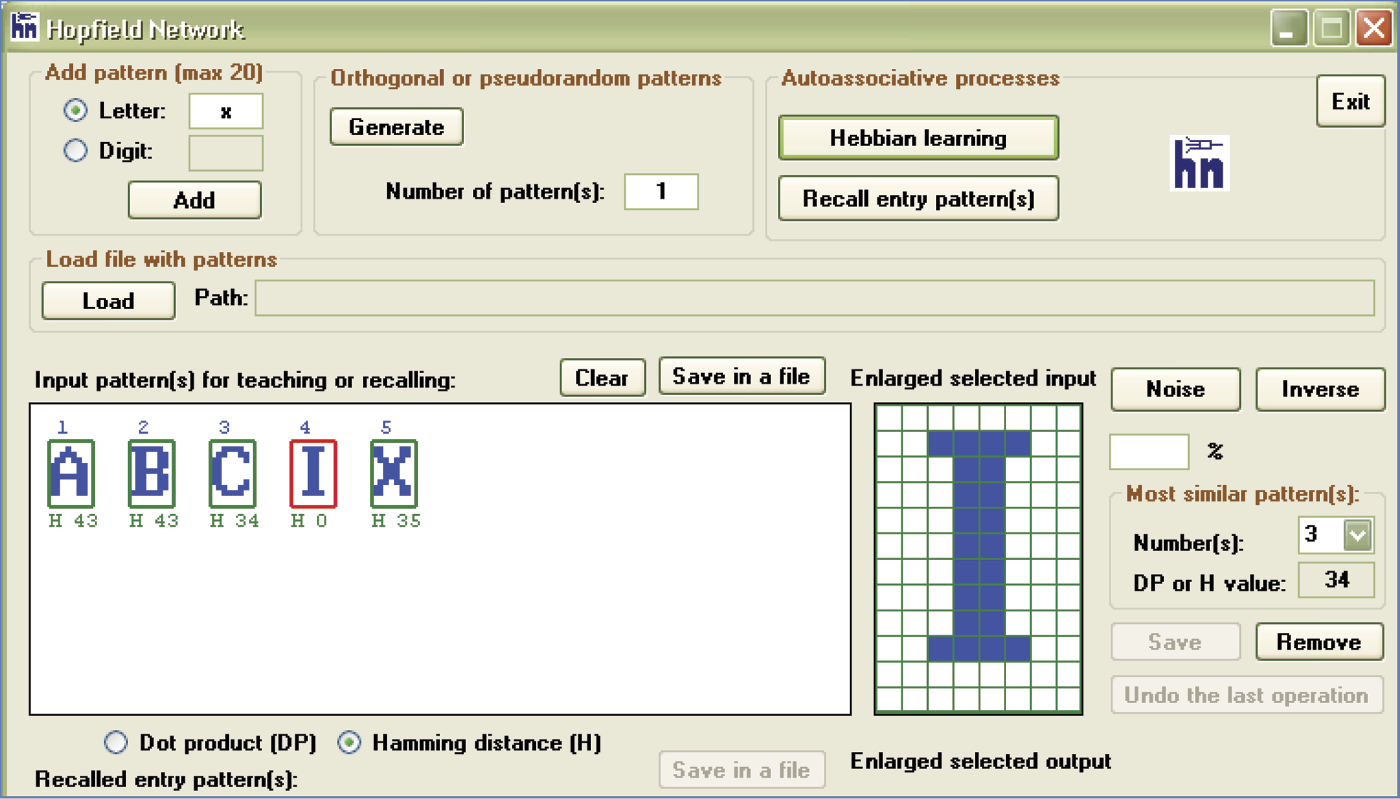
The level of similarity between images can be measured in two ways. The Input pattern(s) window contains two choices: DP (dot product) and H (Hamming distance). DP measures the level of similarity between two pictures. A high DP value for any pattern indicates that it can be confused easily with the currently selected pattern. Hamming distance, as the name indicates, measures the differences between two images. If a pattern produces a high H value, it is not similar to the one selected. A low H value indicates a pattern similar enough to be confused with the current image of choice.
After you select the image to be memorized by the network you want to examine, you can manipulate the pattern. It is easy for a network to recall an image based on an idea but not so easy for it to handle a randomly distorted image. In that situation, a network can demonstrate its associative skills.
Simply indicate in the box on the right marked with the percent symbol (%) the percentage of points of the pattern you want the program to change before it is shown to the network. You can specify any number from 0 to 99 but you must also press the Noise button to specify noise or distortion. You can also challenge the network further by choosing a reversed (negative) image by pressing the Inverse button. The distorted pattern selected will appear in the enlarged selected input window. Can you guess what pattern generated the picture? You can also assess whether your modified pattern has or has not become more similar to one of the competitive images after the changes. You will note the affinity of the distorted pattern with other patterns presented as numbers located below the thumbnail images of all the patterns in the Input pattern(s) window for teaching or recalling.
We suggest you do not set large deformations of the image at the start of teaching because the result will be difficult for the network—and you—to recognize and compare with the original. From our experience, we suggest that distortion not exceed 10%.
Good results are achieved with large numbers of changed points. Although this seems paradoxical, large numbers allow the image to retain its shape; the distinguishing feature is a color change (white on black and vice versa). For example, if you choose 99 as a percentage of the points to change, the image produced is a perfectly accurate negative that contains the same information and can be traced easily in the modeled network.
When changing fewer than 99% of the points, the resulting image will contain minor changes and be recognized by the network without difficulty. However, poor results are achieved when attempting to reproduce the original pattern with distortions ranging from 30 to 70%. The network recalls some information and needs many iterations to reproduce the image. As a result, the process takes a long time and the reconstructed pattern is deficient because it will still show distortions. Figure 11.17 shows a slightly distorted starting image on the left and a strongly distorted starting pattern on the right based on the user’s choice of the percentage of distortion.
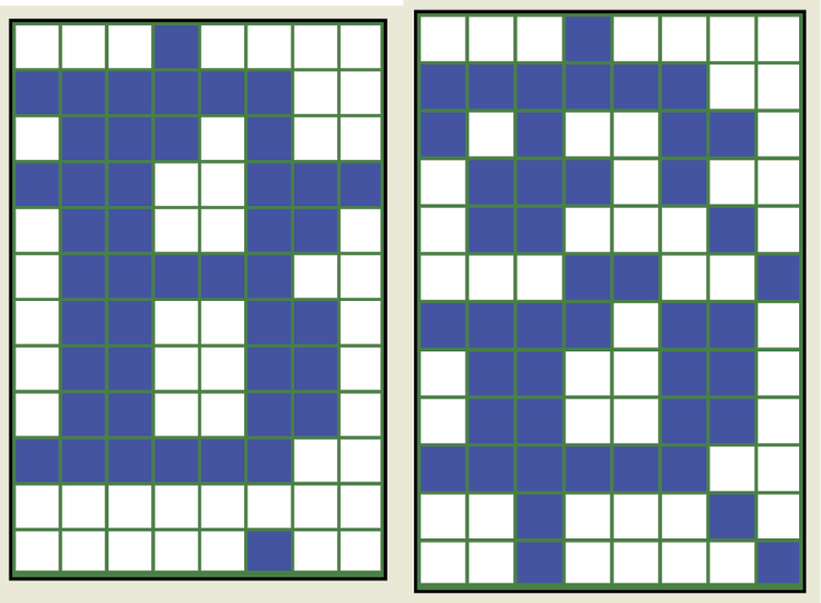
Patterns from which the process of recalling messages stored on the network begins. Left: Less distorted pattern of letter B. Right: Strongly distorted pattern of letter B.
A network remembers a memorized pattern based on signals specified at entry. The neurons transform the signals into new outputs that again by feedback inputs are processed. This process stops automatically when no changes occur in the output signals of an iteration. The stop indicates the network “remembered” the image. Usually the result is the distorted version of the image you applied the network.
If the image that triggers the remembering process is only slightly different from the standard, the result may appear almost immediately, as shown in Figure 11.18. Note how the network recalled the correct shape of the letter B, starting from the distorted pattern in Figure 11.17 (left).
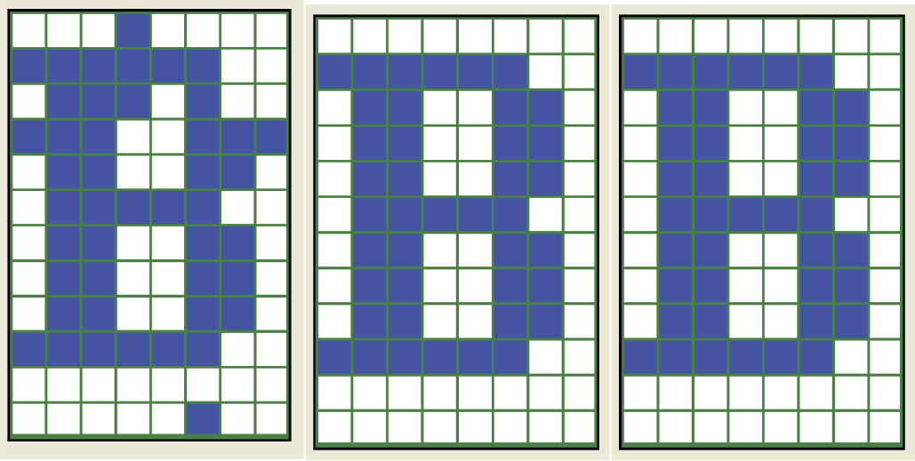
Fast reproduction of a distorted pattern in a Hopfield network working as an associative memory.
Figure 11.18 and the following figures in this chapter show sequential (from left to right) sets of the output signals from the tested network. Figure 11.18 shows that the output of the network reached the desired state by generating an ideal reproduction of the pattern after only one iteration. Slightly more complex processes were introduced. In this case, the network needed two iterations to achieve success (Figure 11.19).
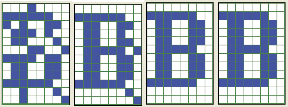
One of the interesting characteristics of a Hopfield network will become clear after you experiment with the program: the network’s ability to store both the original pattern signals and the signals that are negatives of stored patterns. This can be proven mathematically. Each state of network learning that leads to memorizing a pattern automatically creates an attractor corresponding to a negative of the pattern. Therefore, the network can recover a pattern by either finding the original or its negative.
Both images contain exactly the same information (the only difference is that +1 values are converted to –1 values and vice versa). As a result the network’s finding of a negative of distorted pattern is considered a success. For example, Figure 11.20 depicts the reproduction of a heavily distorted pattern of the letter B because the network found that negative.
11.6 Program for Examining Hopfield Network Operations
These results and many more can be observed and analyzed with the Example12b program. The program begins by accepting automatically generated patterns or those a user provides. These patterns that are meant to be remembered by the network are images of digits or letters input via a keyboard or abstract images generated by the system. To maintain the quality of the thumbnails, the associative memory has a limited capacity. Example12b limits the maximum number of input patterns to 20. You can utilize as many patterns as you wish, but in reality constraint works better here. The fewer the patterns, the shorter the learning time. This means the network will work faster after learning and make fewer mistakes.
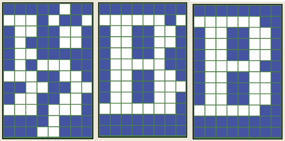
If more than 16 patterns are set, the network starts to combine and over-impose the data because of the limited number of neurons for remembering the patterns provided. The significant errors that result can be observed as crosstalk that appears as artifacts from other patterns in the images generated. This crosstalk effect can be seen in Figure 11.21. Note that in this figure and the following ones, we used a slightly different form of network presentation for Example 12b. From left to right, we show:
- Reproduced pattern without distortion
- Intentionally distorted pattern
- Consecutive steps of reconstruction of pattern by network
This kind of layout will be useful when we start to work with patterns of different shapes. We can compare original patterns on the left with the final outputs of the network on the right.
Figure 11.21 indicates that overloading a network with excessive remembered patterns causes an uncorrectable disturbance of its operation. The disturbance appears as the system attempts to reconstruct a pattern that appears distorted and distinctively different from the original used during learning. This phenomenon can be observed even if the reconstruction process begins with a virtually undisturbed signal (Figure 11.22) because the structure of the character remembered by the network includes permanent memory imprints from other patterns.
Pattern distorted by crosstalk cannot be correctly recalled even if an undamaged version is supplied at input.
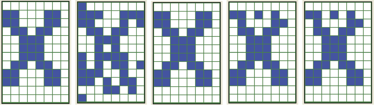
One other interesting phenomenon is illustrated in Figure 11.21. During the first iteration, just after a strongly distorted pattern of letter X was added to the network, the program reconstructed a perfect image of the pattern. However, further processing resulted in distortion of the reconstructed pattern with “echoes” of other pattern memories. This can be related to the real-life experience when you learn (sometimes too late) that the first idea that came to mind was in fact the best. Considering the result from different perspectives led you to realize that your conscious choice was inferior to the initial impulse provided by your intuition.
We should discuss some details of the Example12b algorithm. When executed, the program collects the information to be remembered by the network in the form of patterns and requests a pattern (Figure 11.23) that can (but does not have to) be remembered by the network. The patterns to be remembered may be input in the Add pattern group field. You can add a letter or digit in the proper field, then confirm your choice of letter or digit by clicking the Add button. The selected letter or digit will appear in the Input pattern(s) window for teaching or recalling. Remember that the maximum number of patterns you can add is 20. The program will give you full control over the input patterns. After each digit or character key is pressed, the system will illustrate a precise structure of the image in the Enlarged selected input field.
Inputting data for associative memory with the ability to modify or reject each supplied character.
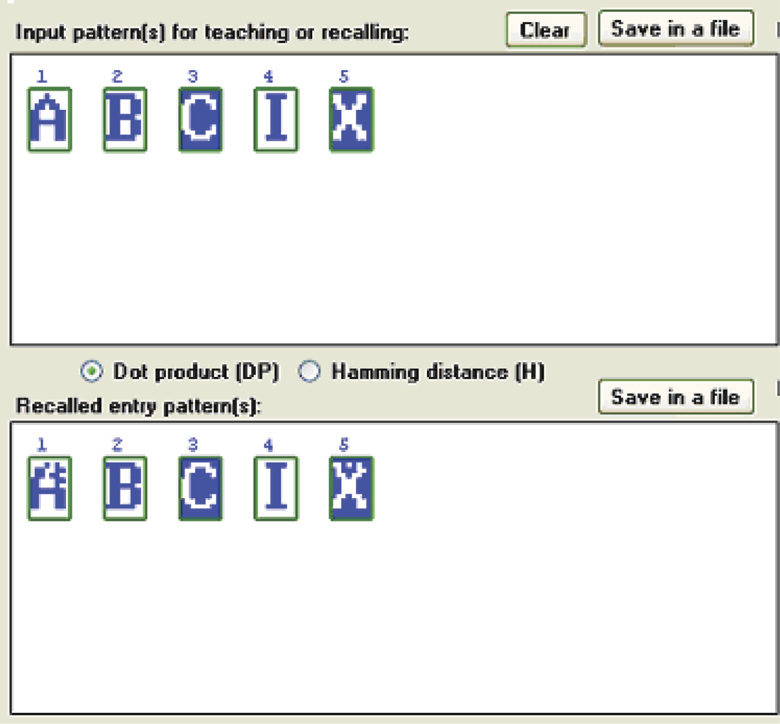
After the patterns to be memorized are input (they will appear in the teaching or recalling dialog window), you can select any of them with a mouse, invert them by clicking Inverse and Save, or remove them from the learning sequence with the Remove button. Removal may be the only option if you find that a pattern is too similar to another input already presented. It is also possible to generate the patterns automatically (discussed later), but the automatic ones tend to have shapes that are difficult to understand. It is advisable to use few of them when you start working with the program. It is best to start with a few letters (e.g., A, B, C, I, X). After entering each letter in the Letter input field, press the Add button.
After you finish inputting and perhaps modifying the pattern sequence to be memorized (presented in the Input pattern(s) window for teaching or recalling), press the Hebbian learning button. You can use this button often, especially when you want to teach a different set of patterns. After the Hebbian learning button is pressed, the Recall entry pattern(s) button will become active almost immediately. It indicates that the learning process has been completed and the network is ready for examination.
You can now verify how the network recalls each memorized pattern. Pressing the Recall entry pattern(s) button when no pattern is selected in the Input pattern(s) for teaching or recalling dialog box will recall each input pattern visible in Input pattern(s); recalled patterns will appear in the Recalled entry pattern(s) window. It is interesting to see how the network memorizes and recalls letter patterns. The example network recalled B very well; performed less well with C, I, and X; and regularly generated crosstalk when recalling A (Figure 11.24).
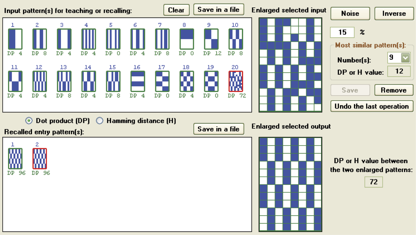
When you click any pattern visible in the Input pattern(s) window, the Noise and Inverse buttons displayed on the right side of the enlarged selected input become active. You can use the input field below the Noise button (labeled with a percent sign) to set the percentage of points in the input pattern to be changed. You can enter any number from 0 to 99. After the Noise button is pressed, the program will randomly change the number of pixels as you requested and insert an enlarged thumbnail of the pattern in the Enlarged selected input window (Figure 11.25). If you then click the Save button under the Enlarged selected input window, this noise-distorted pattern will be inserted into the sequence, which is visible in the Input pattern(s) for teaching or recalling window.
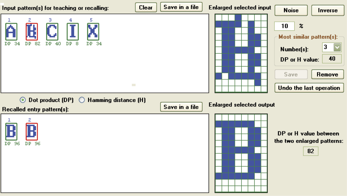
Images available in enlarged selected input and enlarged selected output, and their likelihood metrics (DP or H values between enlarged patterns).
The Inverse button near the Noise button displays a similar behavior. The Inverse button will invert the pattern selected (i.e., blue pixels are changed into white and white pixels into blue). The changes made with the Inverse button must be confirmed in the same way as with the Noise button—by clicking the Save button. The results of saving are identical in both cases. If you want to discard the last change, you can use the Undo button that cancels the last Save operation. It will also cancel the last removal of a pattern via the Remove button. The button titled Undo last operation cancels the previous save or remove action.
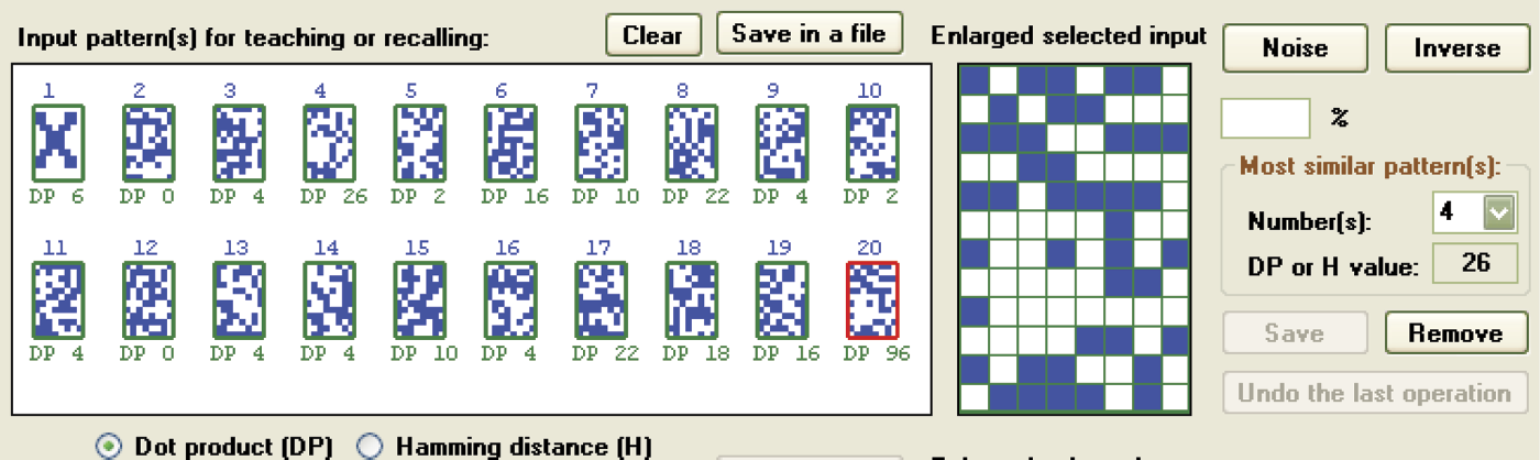
The question of similarity (or lack of it) of the memorized patterns is crucial and we will therefore give it more focus. As noted in our discussion of Figure 11.21 and Figure 11.22, signal patterns sometimes overlap and produce crosstalk. This phenomenon is amplified if the memorized patterns are similar. This is a logical result. With similar patterns, the memory imprints (all located within the same network) tend to overlap tightly. If the same neuron is to output +1 as part of a remembered letter A, sometimes –1 because it is part of a letter B, and +1 for recalling a letter C, the resolution becomes difficult. If the memorized patterns differ greatly, the issue is less serious because fewer conflicting pixels are involved. If the patterns are very much alike, their representations by interconnection weights become so mixed in the neural memory that recalling of any single pattern becomes problematic (Figure 11.26).
If you want to observe the performance of a network under reasonably favorable circumstances, you must invest some effort, at least in the beginning, into providing clearly distinctive patterns. As a result, the program will support you in two ways. First, while inputting new patterns, the program will immediately calculate and provide you with a similarity factor between the new and already memorized patterns. You can then control in real time the effects of pattern overlaps while inputting the characters with a keyboard.
This step is simple because clicking one of the thumbnails of the previously input patterns (visible in the Input pattern(s) for teaching or recalling window) will display the numbers under each of the thumbnails representing similarities between the previously provided patterns and the new one. This similarity can be displayed as dot product (DP), in which case the higher the number, the higher the level of similarity to the already provided pattern. The result can be displayed as Hamming (H) distance, in which case the higher the value, the better because it indicates more distance between the new and previously provided patterns.
Second, the enlarged selected input window will display any pattern you select. On the right side, just under the Noise and Inverse buttons, there is a Most similar pattern(s) field that will display a pattern that most closely resembles the selected one. This field allows you to analyze potential risks because you can see related patterns that may be mistaken for the selected the current one. This number of potentially conflicting patterns will appear in the Numbers field. The input DP (maximum value of scalar product) or H (minimal hamming distance) value will show the chosen similarity value.
11.7 Interesting Examples
We realize that the description of the handling and functioning of the Example 12b program is complex but the work is worth the effort. Our experiments with this program will demonstrate the interesting tasks it can handle and allow you to carry out further studies in areas that interest you.
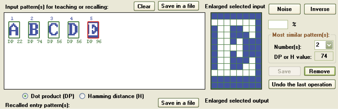
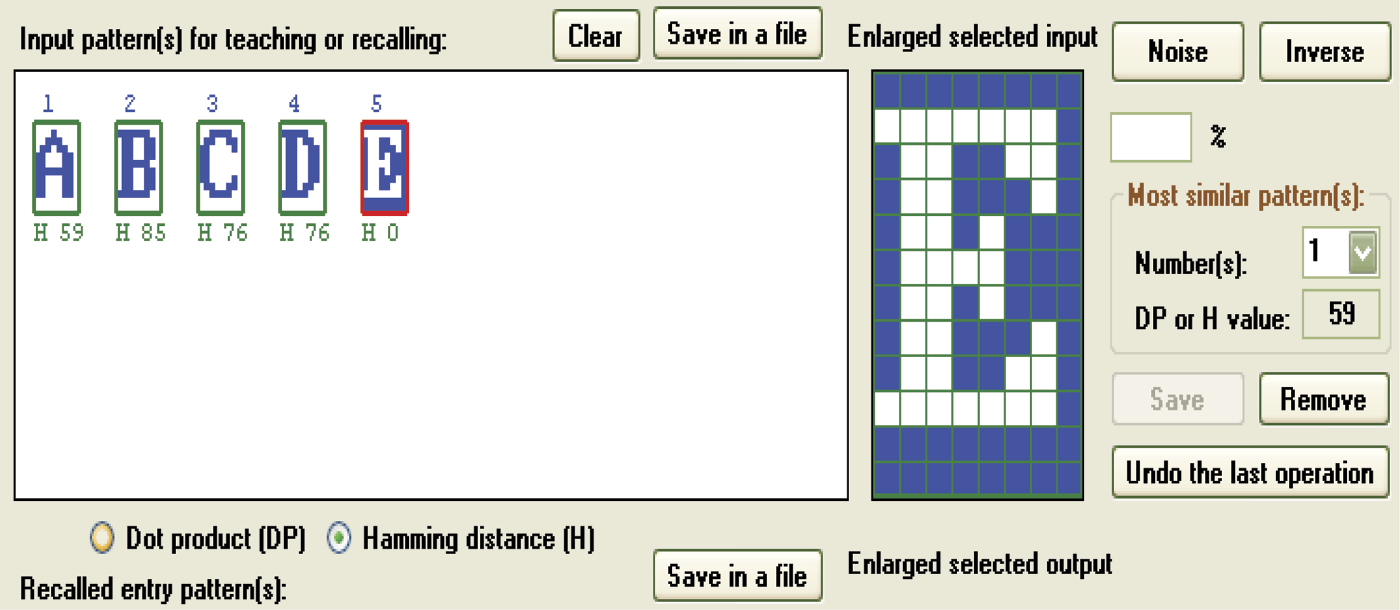
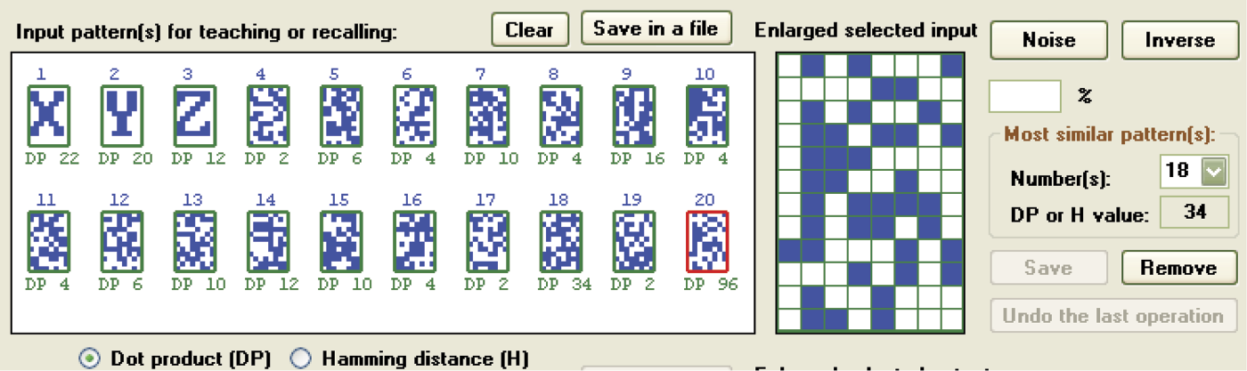
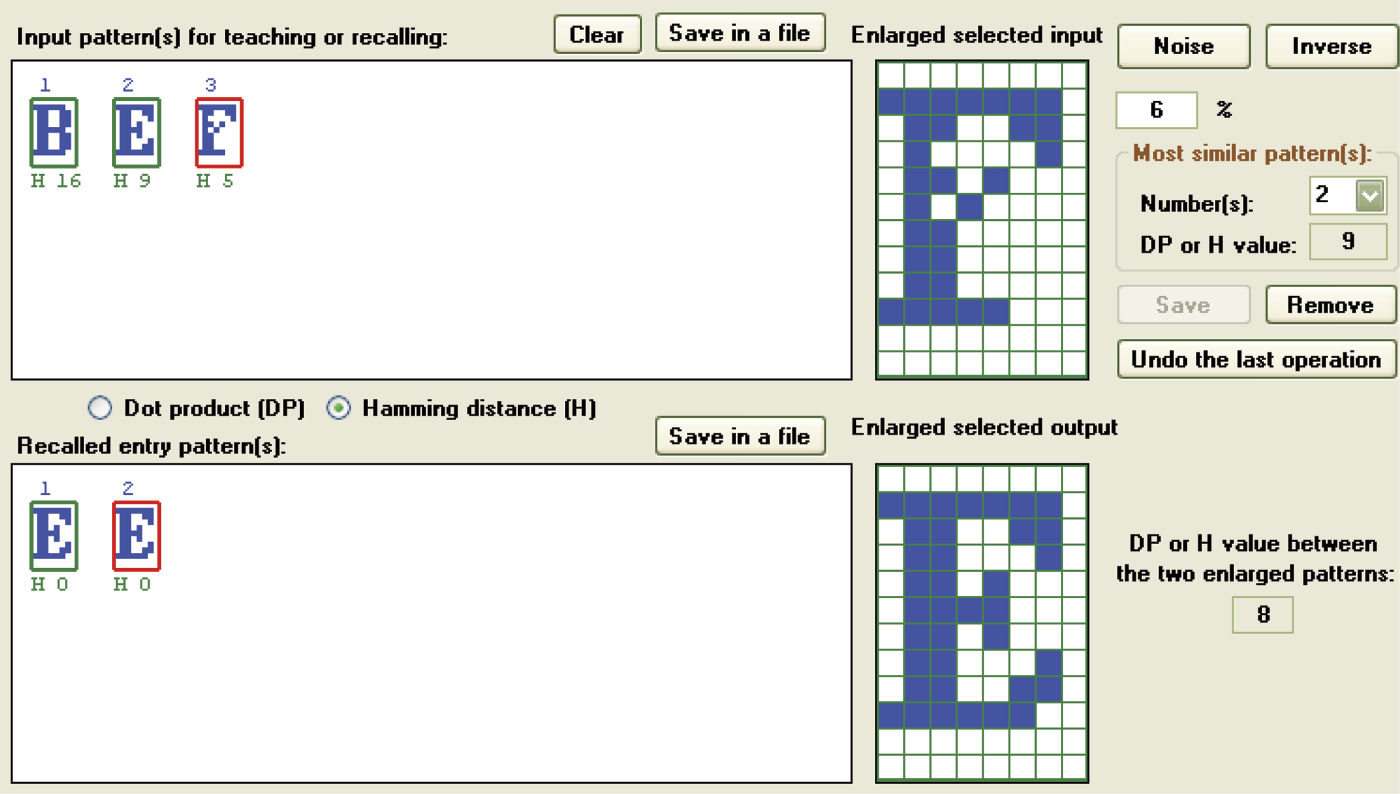
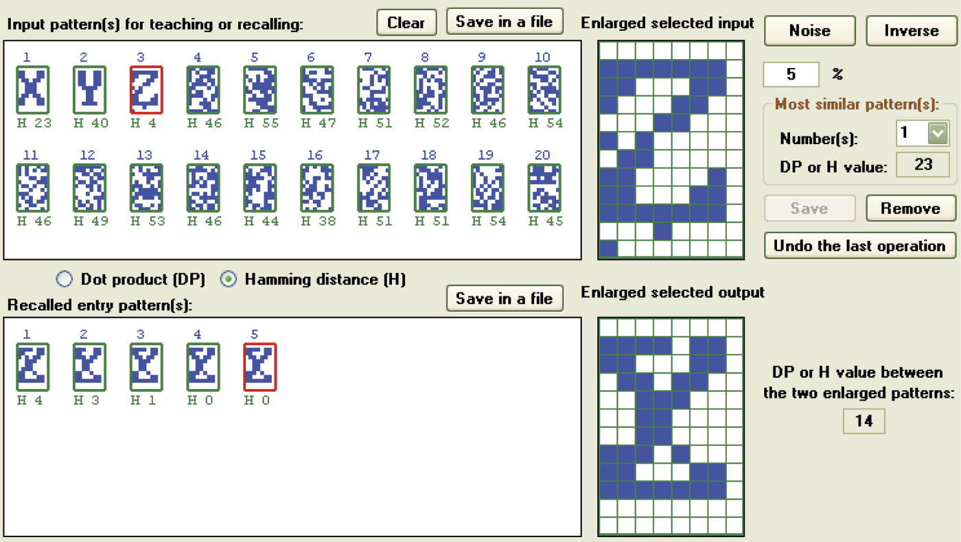
We can analyze the situation presented in Figure 11.27. As seen in the upper section, we already entered patterns A, B, C, and D. The E entry is weakly differentiated in relation to the others. The measure of the similarity of E to the letter A pattern is 22 (a decent result). The strength of the similarity to the letter B is 74 units; strength scores for C and D equal 56 units. At the right side of the window you will see in the Most similar pattern(s) group box how the program warns the user that the entered E pattern will be mistaken for the B pattern. You can then reject the B pattern if you so choose. Using the inversion (negative of the pattern) does not change the similarity values (Figure 11.28).
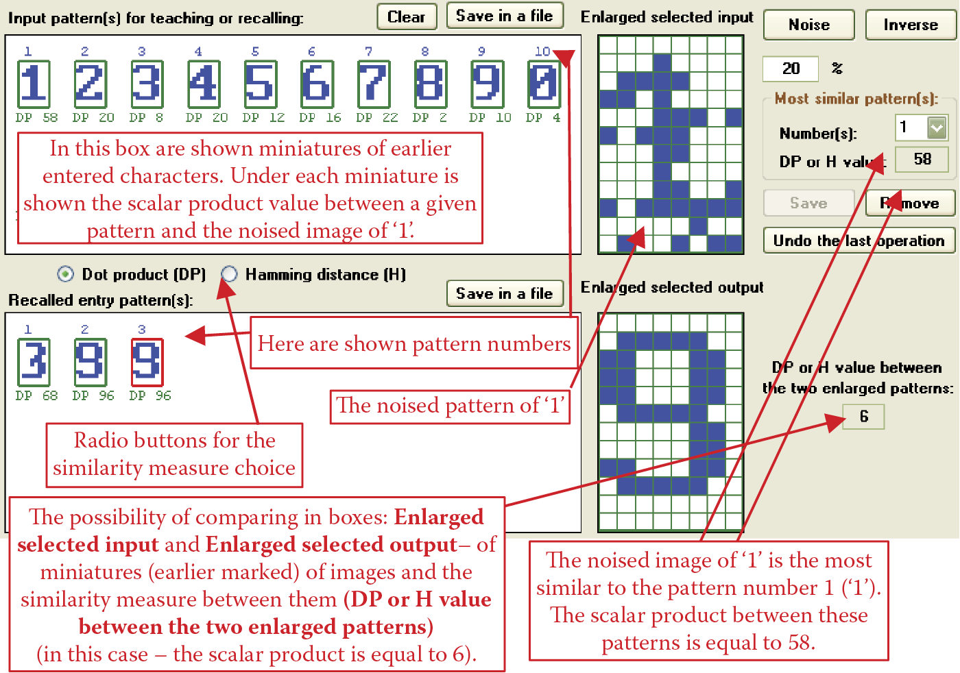
The basic measure of the similarity of a new image to patterns defined earlier is calculated in the program as the dot product (DP) of the vectors describing these signals in the input signal space. More precisely, the absolute value of the scalar product is taken into consideration but you really need not reflect on what it means. The DP is displayed in the appropriate radio at the center of the screen. If you click the Hamming distance (H) button, the program will utilize another way to calculate pattern similarity (Figure 11.29). The chosen measure will be displayed under each pattern miniature.
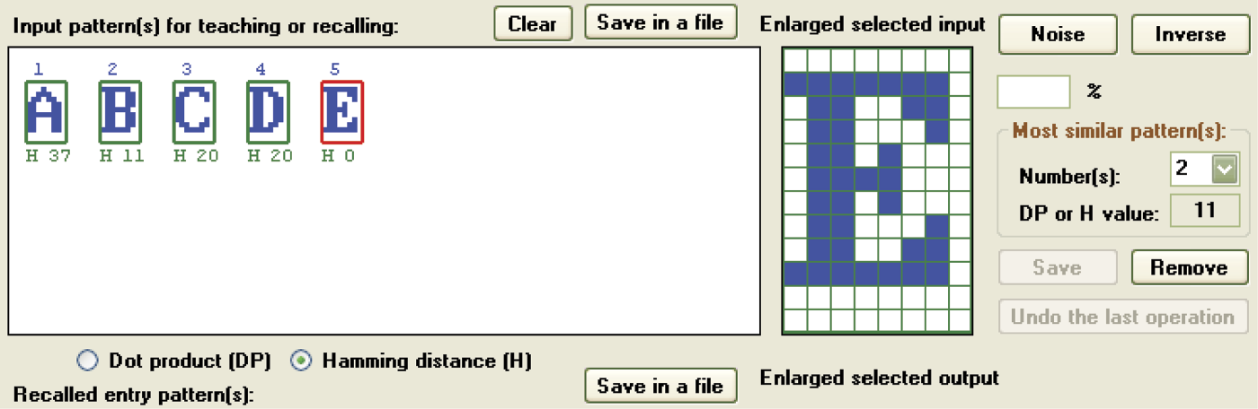
Figure 11.29 shows different values under individual patterns. The pattern that is the most similar shows the least distance. You should know how to interpret this because the Hamming distance (H) measure was selected. You may wonder why the program allows two similarity measurement possibilities. Depending on the result desired, the two measures provide different information and apply to different objectives.
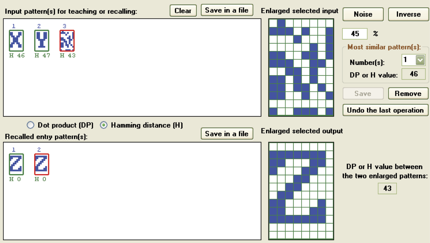
During the generation of new images, it is better to rely on the observation and maximization of the scalar product. The Hamming distance may be misleading because it is sensitive to pattern inversion. Compare Figure 11.30 with Figure 11.27, Figure 11.28, and Figure 11.29 to see what should and should not happen when new patterns are entered.
As you observe a network and track its analysis of patterns, Hamming distance will be a more useful measure. It will allow you to evaluate whether the search is proceeding correctly or the network is moving away from the correct pattern. You may also observe a very interesting phenomenon: the network’s rejection of the correct pattern and acceptance of completely different information (Figure 11.31).
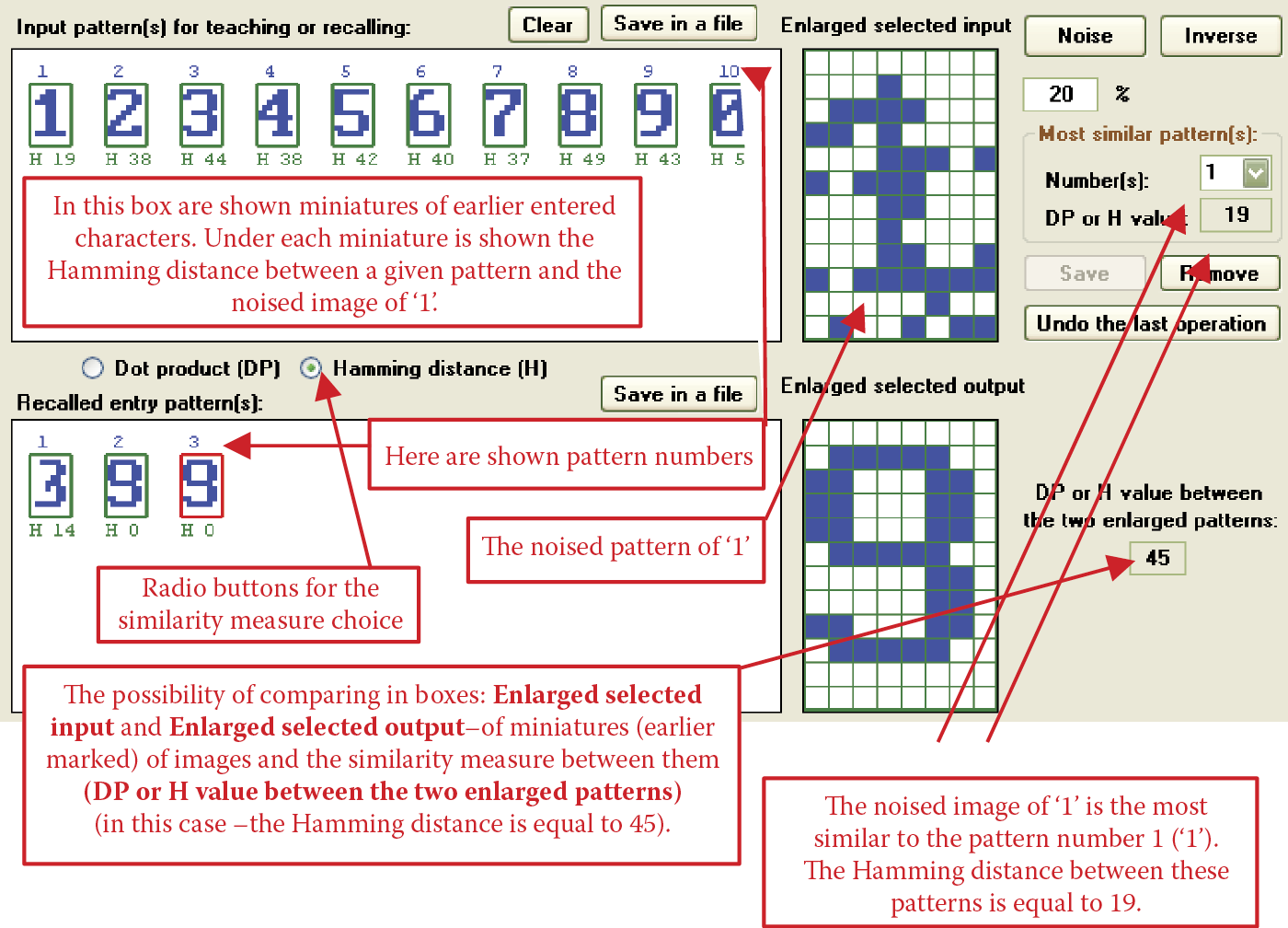
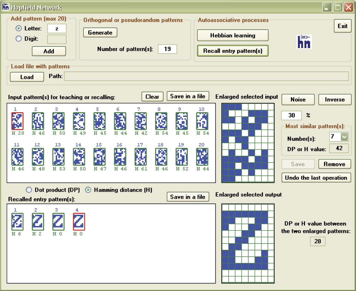
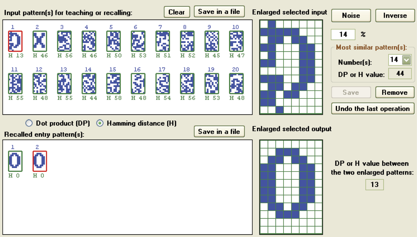
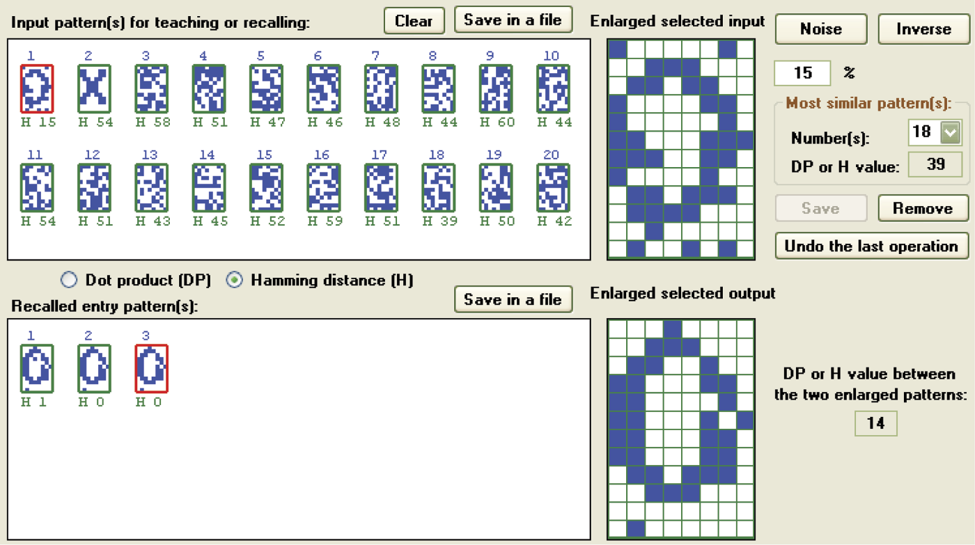
This example corresponds to the situation of entering a disturbed stimulus into the network. For the original signal (1), 20 random changes were performed and the 1 became less similar to its own pattern and also to all the other patterns. This is confirmed by both the signal appearance and Hamming distance values shown. At this moment, the dynamic process of network feedback starts. At first, the network generates an image that dangerously resembles a 3. The network continues to work and generates a 9 pattern.
Note the numbers appearing under the pattern sets in both the Input pattern(s) for teaching or recalling box and the Recalled entry pattern(s) box. They indicate Hamming distances between the signals currently in the network input and all the considered patterns. Hamming distance helps you see which signals correspond to which distance sets. Figure 11.32 shows scalar product values.
Compare the Hamming distance values between the noised 1 pattern and all the patterns in both the input and recalled entry patterns boxes. At the start, the Hamming distance between the correct version of the 1 and the signal shown in the network input is 19. Other patterns are safely distant (37 to 50 units). The program increases distance units if the signal and stimulus are dissimilar (0 and 1) and decreases the units as similarity increases.
You can repeat this experiment easily on your computer. You can generate hundreds of similar results with other patterns and signals. The exercise is worthwhile because you will learn how various combinations produce expected and unexpected results. Experiments performed with a Hopfield network will show you that some patterns can be reconstructed easily and others produce unpredictable or unwanted results (Figure 11.33). In the next section, we will discuss such patterns.
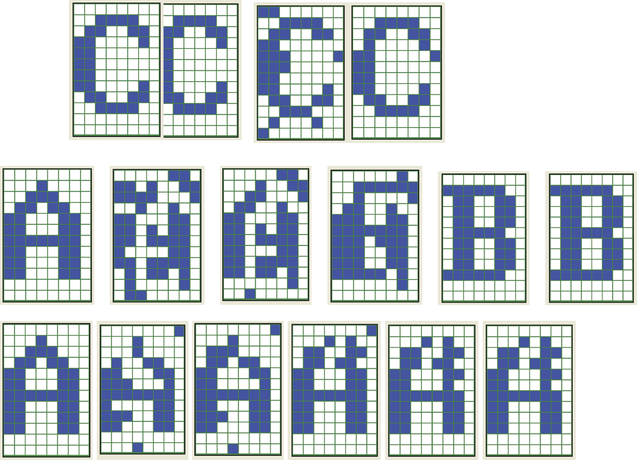
Successful reconstruction of letter C pattern and two reconstruction failures of letter A pattern.
11.8 Automatic Pattern Generation for Hopfield Network
While creating patterns to be memorized by a network, you should observe the value of the scalar product to achieve a set of patterns with minimized crosstalk. You already know that a reasonable set of patterns has DP values as low as possible based on comparison. The ideal solution is to have both patterns display zero scalar product values and is known as orthogonal design. Getting closer to an ideal solution will optimize both learning and network performance.
Creating an orthogonal set of patterns manually is virtually impossible. You can try to get close to the ideal, but you will find out that the images of characters input with a keyboard will always be somehow correlated and their scalar products will not be zeroes. You can, however, delegate this task to the Example12b program that can support you by creating orthogonal patterns without help.
A grouping field for choosing orthogonal and pseudo-random patterns appears in the top part of the screen along with a field that allows you to enter the number of patterns you want the program to generate. Remember to confirm your decision by pressing the Generate button. Also, make sure that the number of patterns you request in the Number of pattern(s) field when added to the number input earlier does not exceed the 20-pattern program limit. Pressing Generate will also produce additional thumbnails of orthogonal patterns (as many as you requested) appearing in the Input pattern(s) window. You can start generating and adding automatically generated patterns from the beginning (Figure 11.34) or try a combined approach by adding one or a few patterns.
If you select all generation of all the patterns at the beginning, the program will create a set of pairwise orthogonal patterns that will improve memory performance greatly. The patterns generated automatically will be simpler and more consistent than patterns entered manually. This is because the patterns generated by a user are pseudo-random, not pairwise orthogonal (Figure 11.35 and Figure 11.36).
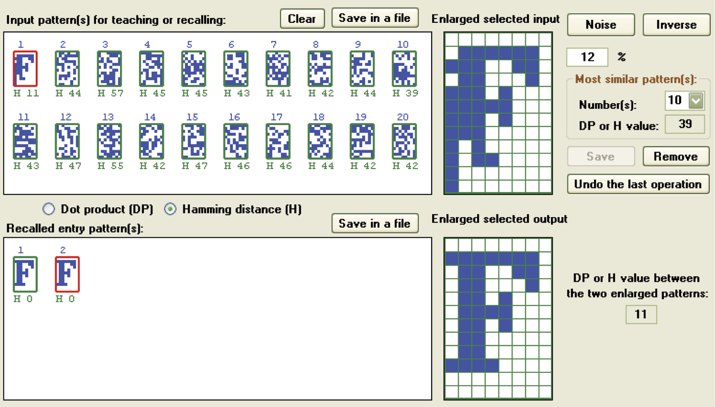
When you enter a character with a keyboard before requesting automated pattern generation, the program will create a number of pseudo-random patterns. You may notice the low values of the scalar products. Orthogonal patterns are very useful when a network works as an associative memory, because orthogonal and also pseudo-random patterns allow reconstruction of the original input image, even if it was severely distorted (Figure 11.37 and Figure 11.38). This, of course, applies to each memorized pattern. However, it is difficult to verify whether a pseudo-random pattern has been correctly reconstructed because these patterns generally appear somewhat exotic.
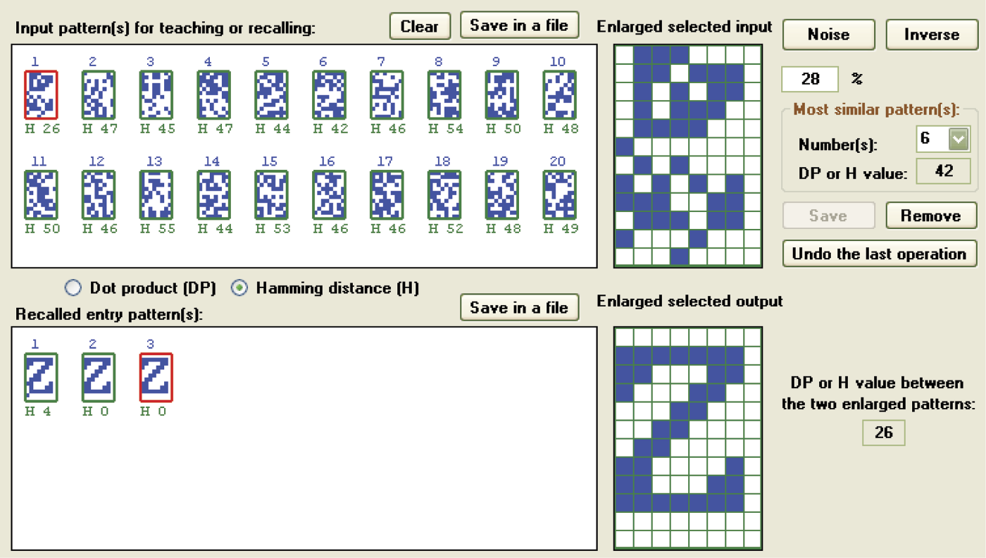
Correct recall of letter Z pattern in which 26 randomly selected pixels (28% noise) were changed.
Reconstruction of correct images with memorized orthogonal or pseudo-random symbols by a Hopfield network, even for severely distorted patterns, has limitations (Figure 11.39 and Figure 11.40). If you distort a pattern too much, the ability to reconstruct it will be lost irretrievably. For example, in Figure 11.38 and Figure 11.40 you can see that a network with pseudo-random patterns can quickly and effectively recall a pattern of a letter Z even 26 and 24 pixels, respectively, were changed.
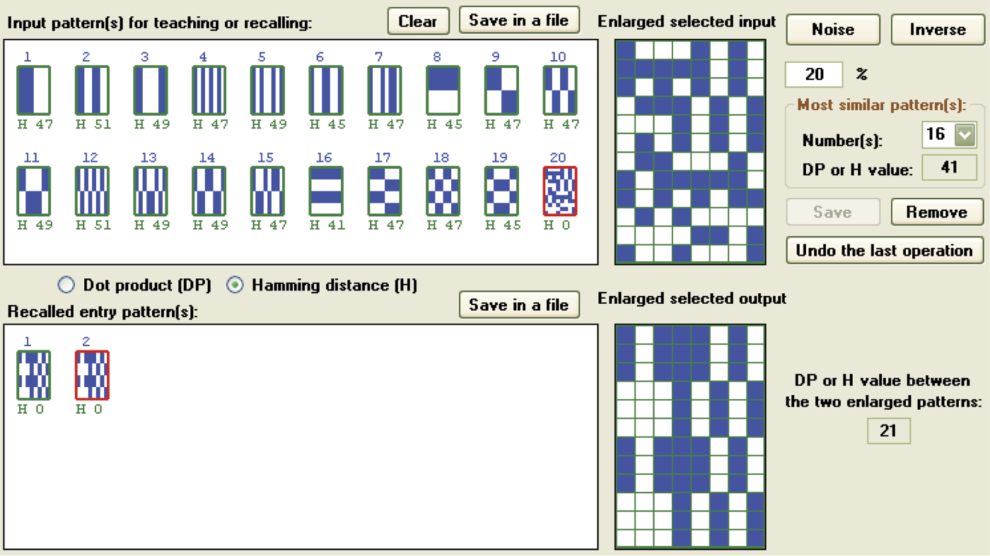
Imperfect recall of orthogonal pattern in which 19 randomly selected pixels (20% noise) were changed.
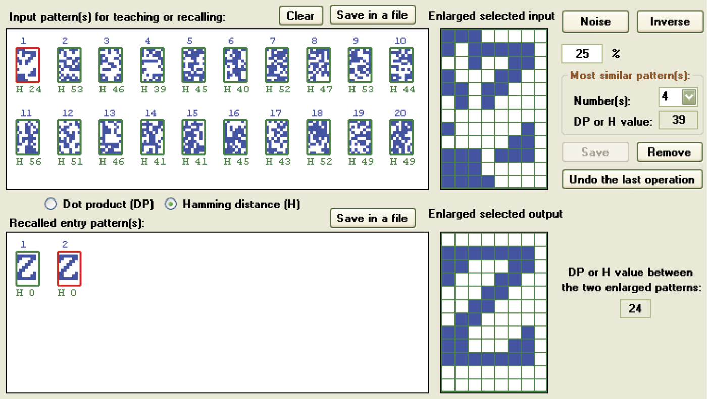
Correct recall of letter Z pattern in which 24 randomly selected pixels (25% noise) were changed.
You can repeat these experiments and a different result will be generated with each attempt, because the distorted patterns will be different and the pixels to be changed will be selected randomly. Quite often, a single pixel difference (e.g., damaging 25 instead of 24 pixels in the original image) will cause inability to reconstruct the image because of the persistent small artifacts that appear in the result (Figure 11.41).
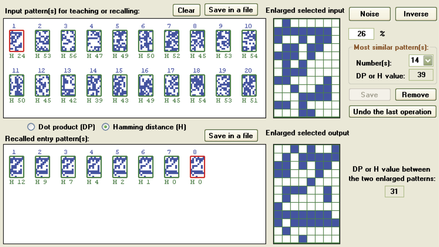
Incorrect recall of letter Z pattern for which 25 randomly selected pixels (26% noise) were changed.
With increased damage to the input pattern, the reconstruction process becomes longer and the final result decreases in quality, until at some point it disintegrates and the network outputs “garbage” only. Even then, it is possible that pure luck may produce heavily distorted patterns that are brilliantly reconstructed (Figure 11.42).
To experiment with a set of patterns that you created and stored on your hard drive, you can use the Load file with patterns grouping field. When the Load button is pressed, a new window display will allow you to select the file with patterns to be loaded into the program. If the file (with a .PTN extension) you provide exists and can be loaded, the program will list it in the editable Path field. The thumbnails of the patterns in the file will appear in the Input pattern(s) for teaching or recalling window.
11.9 Studies of Associative Memory
The Example12b program will enable you to conduct a series of studies that will help you understand the nature of associative memory constructed with a Hopfield network. We have shown you how to inscribe information into the memory and how the information reproduced. Now we will try to describe the capacity of the associative memory constructed with use of the neural networks.
The capacity of a standard RAM or ROM computer memory is limited because all information in the memory is assigned to different locations. You acquire access to certain information by inputting its memory address. The same concept applies to hard disks and CDs. This implies that the information saved in every type of memory is defined precisely by addresses designed for storage. That is why a computer user can determine immediately how much memory is available.
A memory constructed in a Hopfield network follows a different system. It has no specific locations designed to store specific information for memorization or recall. All neurons are engaged in learning a certain pattern. This implies that the patterns must overlap in specific neurons and can cause a problem known as overhearing.
A method of information recall (reading) from a neural memory differs from the method used in standard computers. Instead of indicating the name of a variable that contains certain information or indicating a file name (both methods refer to addresses) to access data, a user can give an associative memory incomplete or distorted information and still receive a suitable answer. For this reason it is almost impossible to determine an upper limit of messages that may be introduced into a neural network.
Obviously, we want a precise theory that explains all these issues in detail. One of the authors wrote a book titled Neural Networks that you may find helpful. The aim of the present book is to introduce elementary concepts of neural networks by experimenting with them. Conducting experiments will help you understand the capacities of neural networks. We can attempt to give you the most practical information on the subject but your experimentation will be the best path to thorough understanding of neural networks.
The first and primary factor determining the simplicity and reliability of recalling memorized signals is the amount of data recorded in the network in the form of memory traces. After memorizing relatively small numbers of patterns (e.g., three), recall of information is reliable even in the presence of significant distortions (Figure 11.43). However, the results of recall depend also on differences in memorized information. Figure 11.44 depicts an experiment conducted on a network with a small number of patterns with high degrees of similarity that led to improper recalls.
If you intend to examine maximum network capacity, you should operate with highly differentiated signals. The most desirable are orthogonal or pseudo-random signals. Only then you can achieve good results even with maximum number of patterns (20 in the example program; see Figure 11.45).
Proper reconstruction of destroyed input signal when maximum pseudo-random patterns are used.
With non-perfect orthogonal patterns (e.g., pseudo-random patterns that emerge if you choose automatic generation after selecting two signals), the results may be acceptable. This will happen only if you select very different initial signals with relatively small distortions (Figure 11.46). Application of more distorted entries will reveal strong overhearing (Figure 11.47).
Success achieved when the network remembers large numbers of non-exact orthogonal patterns.
Proper recall of patterns in a system utilizing orthogonal or nearly orthogonal signals may be affected by large numbers of memorized signals (e.g., entrance images are far more numerous than memorized signals). Even though most patterns in Figure 11.48 are non-orthogonal (and the remainder are orthogonal), the network produced undesirable overhearing; it happens even in cases of insignificant deformations of entrance signals.
Overhearing observed for a minimally destroyed input signal if remembered patterns are not orthogonal.
11.10 Other Observations of Associative Memory
Remembering the correct form of a network model based on a deformed structure introduced as an input is a dynamic process, resembling that in a single-element network and presented in the Example12a program. The next steps in this process are displayed on the screen in the form of images. You can view how the distorted image in the Recalled entry pattern(s) window slowly emerges from the chaos. You can click on any image and track the number that indicates degree of similarity between images produced by the network and individual patterns to view the progress as the network selects the correct images.
The Example12b program allows you to study the use of scalar products and Hamming distance. Both data entry and image reconstruction operations can be performed by pressing proper buttons (without modifying parameters) to switch from a display of scalar products (dot product or DP) to the Hamming distance (H) display and vice versa.
You can use these tools to observe qualitatively and quantitatively how the network-generated approximations of images change their distances from stored patterns and how the values of scalar products change. Some interpretations of results require mathematical knowledge. However, even without it, we can understand the dynamics of the knowledge recovery process in associative memories and the change processes and neuron outputs in Hopfield networks.
The Example12b program also gives you tools for tracking pattern recovery and differentiating steps of the processes. The various choices allow a user to monitor the measures of similarities of patterns expressed as scalar product or Hamming distance. As we follow the network processes of extracting images, we can see what the network does and why. Complete understanding, however, requires considerable patience and work. The memory trace ends only when the next iteration reaches a steady state (i.e., introduces no more amendments to the image). The process can be stopped when oscillations appear.
The “jumping” of a network is interesting. Instead of improving the correct pattern reconstruction, the network suddenly associates a deformed image with a completely different pattern and starts to clean and polish its result (Figure 11.32). A network may create an entirely new idea (non-existent pattern) that represents a hybrid of existing elements combined in an extraordinary and unrealistic way (Figure 11.27)—snakes with wings or dogs with three heads. In our network, we have utilized only pieces of letter images, but they were sufficient to demonstrate how neural networks operate differently and more imaginatively than regular (and dull) algorithms. You can discover other network phenomena by working with the program. Good luck!
Questions and Self-Study Tasks
1. Describe briefly (10 sentences maximum) all the differences between a feed-forward neural network and a neural network having feedback.
2. Develop a formula for predicting the stable output value of the network simulated by the Example 12 program with different parameters (coefficients of synaptic weights), and different values of input signals. How do your results compare with the results obtained with simulations?
3. Read an article from a website or a book on chaos theory. How are this theory and the phenomena described in it related to the issues of recursive neural networks?
4. Research publications and/or the Internet for information about time-varying electrical potentials (electroencephalograms or EEGs) of the human brain. Do you think that these signals indicate the lack of feedback in the human brain or the opposite?
5. Consider whether the human memory (surely an associative memory) is analogous to the crosstalk phenomenon appearing in a Hopfield network? If so, how are they perceived and evaluated subjectively?
6. Based on experiments, determine which similarity measures (dot product or Hamming) can better predict which patterns will be reproduced well by a network and which will pose problems?
7. A relationship that may be derived mathematically exists between the number of neurons in a Hopfield network and the number of patterns that can be efficiently stored with a minimum probability of cross-talk. We know that the more neurons a neural network has, the more patterns it can remember even though each individual pattern involves all neurons across the network. Relate this to the human brain memory that contains about 100 billion neurons. How can you explain the fact that some people have better memories than others?
8. The Hopfield networks discussed in this book were all auto-associative. They formed associative memories that were used to play back memorized patterns. Hetero-associative memory is capable of memorizing associations of different patterns. What scheme must a network have to utilize hetero-associative memory (e.g., the images of objects and first letters of the names of objects)?
9. In this chapter, we used Hopfield networks for very primitive patterns that involved only simplified outlines of letters and numbers. Undoubtedly, it would be far more interesting to work with a network that could operate with images similar to those in Figure 11.13. Why has this not been done?
10. When building a large Hopfield network consisting of many neurons, computer resources are being consumed very quickly. Why does this occur and which resources are affected?
11. Advanced exercise: Build a version of the Example12 program in which the output values produced at the output after the consecutive steps of the simulation are shown in the form of a figure instead of a table. This program should show the time course of the network output values in graphical form (as a chart). What was the main difficulty that had to be overcome?
12. Advanced exercise: Build a version of Example12b in which arrays of neurons representing various stored images will be significantly larger (e.g., increased three times in each direction). Using this improved tool, perform similar experiments as described in this chapter. Compare the observations from such experiments with the statement in Question 7.
* Auto-association is a network working mode that associates a specific message with itself. The application of auto-association to even small fragments of stored information (e.g., images) reproduces the information in the memory completely and includes all the details. An alternative is hetero-association that allows one message (e.g., a photograph of a grandmother) to trigger memories of other information (the taste of a jam she prepared). A Hopfield network can operate with auto-associative or hetero-associative memory. The auto-associative method is simpler and we will focus on it.