
Chapter 10
Self-Organizing Neural Networks
10.1 Structure of Neural Network to Create Mappings Resulting from Self-Organizing
To this point, we demonstrated that neural networks can be taught by teachers or learned independently. We will now talk about networks that teach themselves without teachers and agree based on the interactions to handle the functioning of all neurons so that their cumulative results take on some new quality. These systems automatically generate complex mapping by transforming a set of input signals into output signals. This mapping generally cannot be predicted or controlled. Thus these networks are far more self-reliant and independent than the networks described earlier in this book.
The creator of such a network can impose only slight control over the properties. The essence of their operation and the final mapping depends on the results of their functioning. The actions of such networks are determined mostly by a process of self-organization. Details of the process will be illustrated later in this chapter. Before that, we will briefly explain various applications of self-organizing neural networks because they serve as serious tools for serious purposes.
Mapping is a rich and complex mathematical concept that exhibits several specific properties. We intend to discuss important ideas without burdening you with theory. Some important details are admittedly complex, but they will prepare you to build and work with self-organizing networks and take advantage of their unique properties. We assume that you are an eager adventurer willing to explore difficult issues if you have read this far.
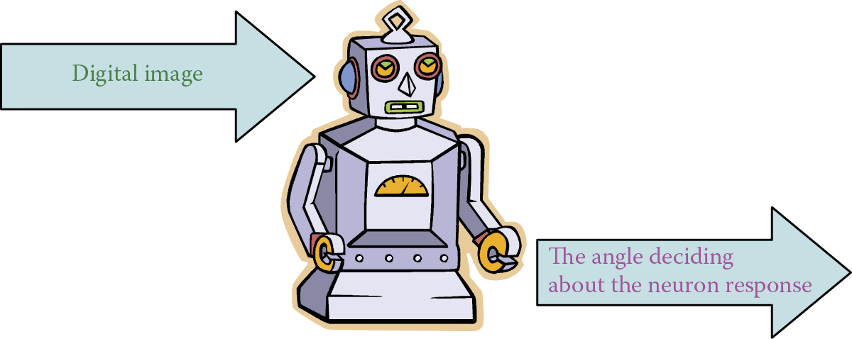
We often must convert signals from input to output according to certain rules. When building a robot to perform certain tasks, we must ensure that it can convert the input signals received by sensors (video cameras, microphones, touch replacement contact switches, ultrasonic sensors, approximation sensors, etc.) correctly to control the signals for actuator devices driving the mechanisms that operate legs, graspers, arms, and so on (Figure 10.1). The conversion of input signals into correct output signals is called mapping (Figure 10.2).
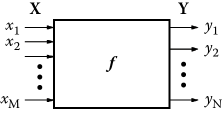
Of course, a simple random mapping would be useless. Mapping is crucial because it ensures that a robot moves correctly, performs meaningful tasks, and responds properly to commands. The mapping binds stimuli recorded by sensors to concrete moves performed by actuators. Thus mapping must be properly designed and programmed correctly. Engineers who design robots and other sophisticated devices work hard on mapping because mapping is an essential component of the “brain” that controls a robot. Mapping is simple if a system has only one input signal and one output signal.
However, even the simplest robot involves many sensors and actions, and mapping becomes a difficult and demanding task. Attempting to program the mappings for complex tasks manually would require more time than an average human life span.
This is where self-organizing neural networks prove useful. Figure 10.3 illustrates such a network structure. Self-organizing networks usually have several inputs. Figure 10.3 shows only three so we can keep the illustration simple. A tangle of connections of 30 inputs would be impossible to trace in a diagram. However, self-organizing networks in practice usually involve more than a dozen inputs. This number is usually more efficient in various applications than networks utilizing far more signals.
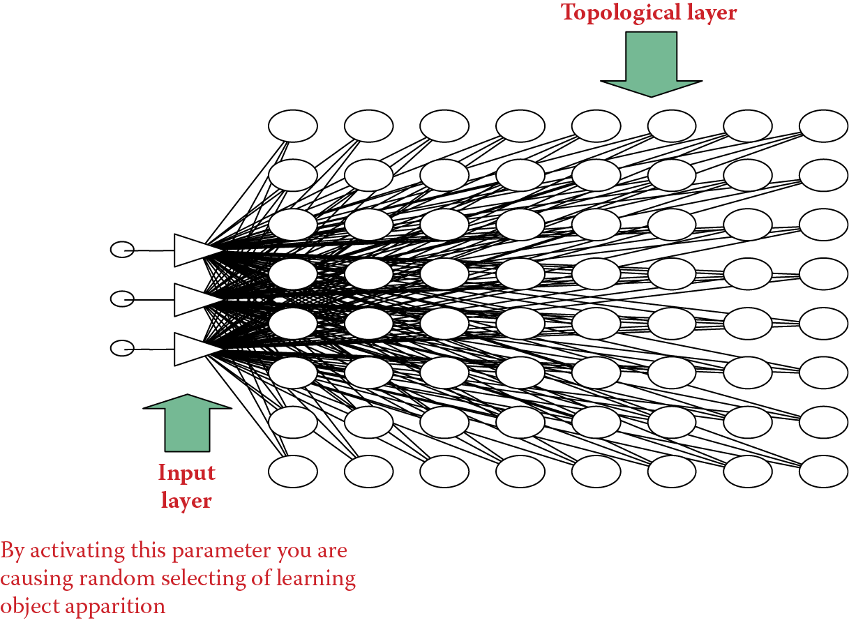
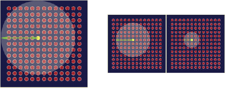
A more important issue is that these networks tend to generate more outputs because of vast numbers of neurons that form the so-called topological layer. “Vast numbers” means at tens to thousands of neurons. These networks are far larger and more flexible than all the networks discussed to this point and we should understand the topological layer and what it does. We described the concepts of rivalry and “winner” neurons in an earlier chapter. Because they are also useful for this discussion, a brief review is in order. After providing specific input signals to the network, all the topological layer neurons calculate their output signals in response to the input signals. One signal in the group is the largest and the neuron that produced it becomes the winner (Figure 10.4).

Example distribution of output signal values presented on topological layer of network with selected signal from “winner” neuron.
Self-organization identifies one and only one winning neuron. Thus the predominance of the winner among the competitors is clear. In exceptional cases, a network may generate a completely abnormal input signal (not included in teaching set) after self-organization. Determining the winner in such cases is difficult because all the topological layer neurons produce very weak but consistent signals.
10.2 Uses of Self-Organization
Self-organizing networks form certain representations of a set of input signals into a set of output signals based on certain general criteria. The networks perform this task independently, solely on the basis of observations of input data. The representation is no way determined in advance by the network’s creator or user. The structure and properties arise spontaneously in a coordinated self-learning process involving all the elements of the network.
This spontaneous creation of signal projection is called self-organization. It is another form of self-learning from a different view. The effects from the program used in this chapter will be interesting. Self-organization involves an obviously higher level of network adaptation of a network by optimizing the parameters of each neuron separately. The coordination of activities of neurons contributes produces highly desirable grouping effects.
The grouping effect results when a network in the process of self-organization tries to divide the input data based on certain classes of similarities. The groups are detected automatically among the input objects (described by the input signals) and the system places similar signals in an appropriate group. The signals for each group are distinctly different from the signals assigned to other groups.
Such data clustering is very useful in many applications. A number of specialized mathematical techniques involving the analysis and the creation of such groups were developed and they constitute the specialty of cluster analysis. These analysis methods are useful in various business applications, for example, comparing similar companies in an effort to predict their returns on investments. The methods can be used in medicine for studying disease symptoms to determine whether they are indicative of a known or unknown disease.
Figure 10.5 depicts an example of a neural network that can group input signals (color image pixels coded as the usual red, blue, or green components) according to similarities of their colors. Figure 10.6 shows the effect of the network before self-organization (left) and afterward (right). The figure was created in such a way that in every place where there is a topological layer neuron, was drawn a box filled with such color of the pixel input, which makes this particular neuron able to become a “winner.”

Network grouping input signals (components corresponding to typical coding of digital image) in collections indicated by different colors.

Figure 10.6 (left) shows the activity projection of the network before self-organization. The figure at right shows the process. Grouping image pixels of similar color is not a task that yields special benefits. You may view Figure 10.6 and ask why such a feature is needed. The answer is in Figure 10.7 depicting topological layer of a self-organizing network programmed to compare data of different companies.

Network inputs cover type of business, capital owned, number of employees, accounting data reflecting profits and losses, and other parameters. The network grouped these companies and so placed the parameters that each neuron wanted to become the winner when information about its company was shown. A year later, the companies were analyzed again. Some produced losses or were threatened with bankruptcy. Those neurons are shown in red on Figure 10.7. Other companies suffered economic stagnation. The neurons assigned to them via self-organization are indicated in blue in the figure. Finally, companies that yielded optimistic results are shown in green.
You may find plenty of impressive examples of self-organization like this on the Internet. You can input “self-organizing network” or “SOM” (self-organizing map) on Google and you will find a lot of information about grouping input data into similar classes and practical applications.
Neural networks engaged in self-organization are very attractive tools for grouping input data and creating similarity classes among them. The attractiveness of the neural approach is mainly that self-organization can proceed automatically and spontaneously. The network creator does not have to provide clues. The necessary information is contained in the same input data from which the network will extract the observation that some inputs are similar and some are not.
After a network learns how to cluster input data, it produces useful results. Winning neurons that specialize in identifying specific classes of input signals act both as detectors and indicators. Now that we understand the effect of clustering in self-organizing neural networks, we will briefly consider the collectivity of network activity.
The networks in which the self-organization takes place are organized so that an image a neuron identifies depends to a large extent on what other neurons located in its vicinity identify. In this way, a community (or collective) of neurons can process information more fully than any one of the individual neurons could (Figure 10.8).

The figure shows the results of our research related to the recognition by a self-organizing neural network of simple geometrical figures shown to it as images. It indicates places where the network independently placed the neurons indicating the various shapes of figures shown to it. A brief tour of this map will reveal that this distribution of neurons is not accidental.
We start with red arrows from the neuron that becomes the winner whenever a square is shown to the network. Nearby are the neurons indicating pentagons; a little farther away are those signaling octagons. This is correct because a pentagon is more similar to a square than an octagon. The neurons recognizing circles are placed near those recognizing octagons and a short path leads to neurons signaling an ellipse, not far from the neuron that understands a semicircle. This neuron has a clear affinity for a segment of a circle (sector) whose shape is similar to that of a triangle.
The workings of collective self-organized networks are interesting and lead us to broader considerations. A community of appropriately linked and cooperative elements makes it possible to discover new forms of behaviors and actions that reveal far more information than individual elements. The same dynamic appears in entomology. A single insect is intellectually primitive and tiny. However, communities of insects are capable of complex, deliberate, and intelligent actions, for example, constructing bee colonies, complex nests, and termite mounds.
Self-organizing networks are convenient and valuable tools and also interesting research subjects. You can master the details of the self-organization processes of neural networks by studying the material in this chapter and performing experiments with the program devised for this purpose. The key concept for understanding and using self-organized networks is the formation of neuron neighborhoods.
10.3 Implementing Neighborhood in Networks
To understand the structure and function of a self-organizing network completely, we had to analyze its functioning and compare its performance with those of simple self-learning networks described in Chapter 9. We learned that the overwhelming influence of random initial values on the course of simple self-learning means that the creator of the network does not control what the neurons will learn.
After completing self-learning, the distributions of neurons may signal events that may not conform to the user’s wishes. Applying manual intervention to influence self-organizing network behavior is difficult and also contradicts the principle on which such networks are based. The introduction of competition into a network may cause some neurons with adequate inborn abilities to be amenable to the teaching process; the others will resist it. This dynamic can be seen in Example 10c.
The program outputs results that include identification of “winner” neurons for each class that later advance to become detectors. The numbers appear chaotic and seem to have no relation to the locations of detected objects. Thus, the assignment of specific object detection functions to specific neurons may increase or decrease the utility of a network. If, for example, some of the input signals are similar, you may want their appearance signaled by neighboring neurons in the network. A self-organizing network works as shown in Figure 10.8. Pure self-learning networks do not require interference; users can simply accept what will happen.
A solution to these issues is to introduce a new mechanism: neighborhood. Teuvo Kohonen of Finland first applied the neighborhood concept to neurons in networks in the 1970s. Subsequently, networks utilizing neuron neighborhoods and competition became known as Kohonen neural networks.
We will now demonstrate how neighborhood works and what benefits it provides. To date, we have considered neurons in networks as largely independent units. Although they were linked together and transferred signals to each other, their relative positions in the layers did not matter. The numbering of neurons was introduced solely for ordering purposes for organizing calculations in programs simulating networks.
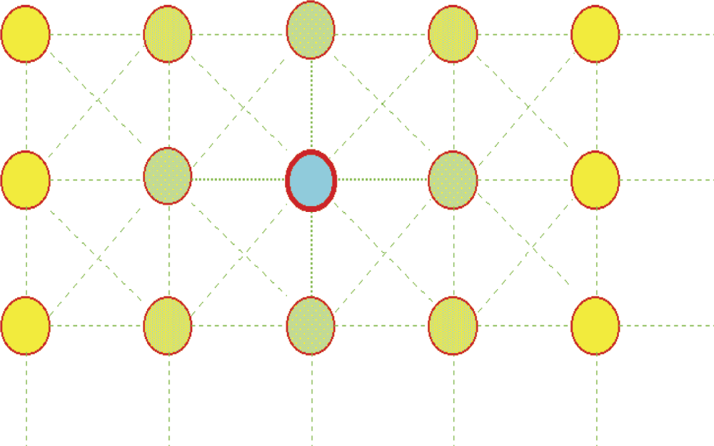
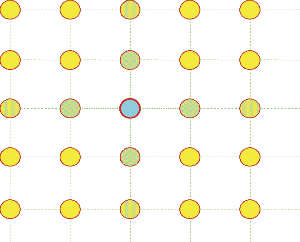
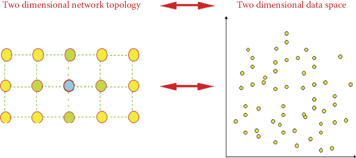
The self-organizing network described in this section is important. The adjacent nature of neurons in the topological layer significantly influences the behavior of the entire network. We usually associate neurons of a topological layer with points of some map displayed on a computer screen—typically a two-dimensional neighborhood. Neurons are depicted as if they were placed in nodes of a regular grid composed of rows and columns. Each neuron in such a grid has at least four neighbors [two horizontal (left and right) and two vertical (top and bottom)] as illustrated in Figure 10.9.

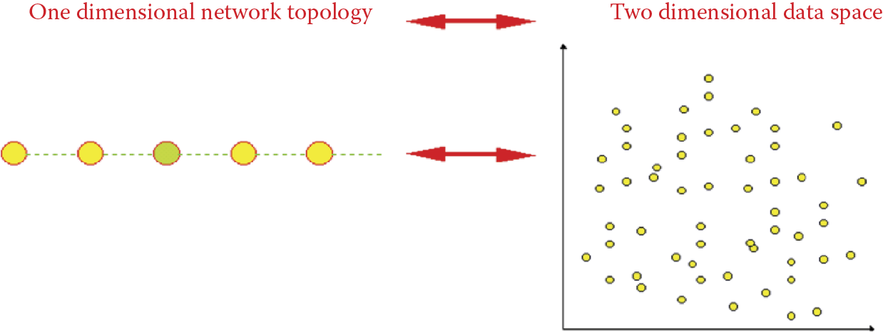
If required, a neighborhood can be considered more broadly by admitting neurons on the diagonal (Figure 10.10) or neurons located in more distant rows or columns (Figure 10.11). The choice of type of neighborhood is entirely up to the user. For example, you can describe a network of one-dimensional neurons that will form a long chain. As shown in Figure 10.12, each neuron will have the neighbors preceding and following it along a chain.

Specialized applications of self-organizing networks may even involve three-dimensional neighborhoods. Neighboring neurons look like atoms in the crystal lattices frequently appearing in textbooks. A neighborhood can include four, five, or more dimensions but the two-dimension type is definitely the most practical and for that reason we will limit our discussion to that type.
A neighborhood consists of all the neurons in a network. Each neuron has a set of neighbors, and in turn it acts as a neighbor to other neurons. Only neurons located at the edge of the network do not have full sets of neighbors. However, sometimes this can be remedied by a special arrangement, for example, a network may be “closed” in such a way that the neurons of the upper edge are treated as neighbors to neurons from the lower edge. Similarly, closings can be applied using the left and right edges.
10.4 Neighbor Neurons
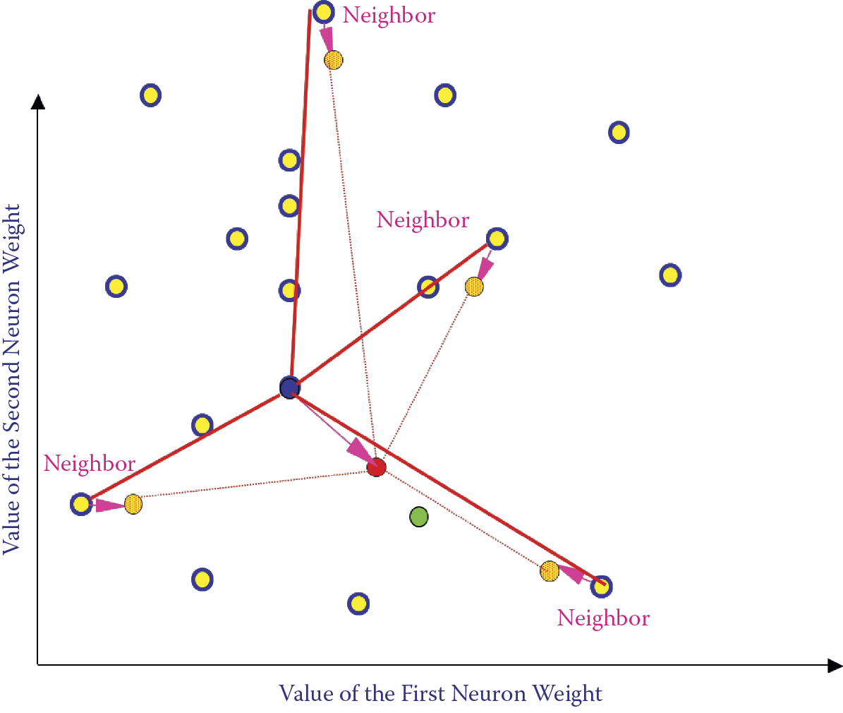
Adjacent neurons (neighbors) play an important role in network learning. When a neuron becomes a winner and undergoes teaching, its neighbors are also taught as we will explain later. Figure 10.13 depicts the self-learning process for a single neuron in a self-learning network.
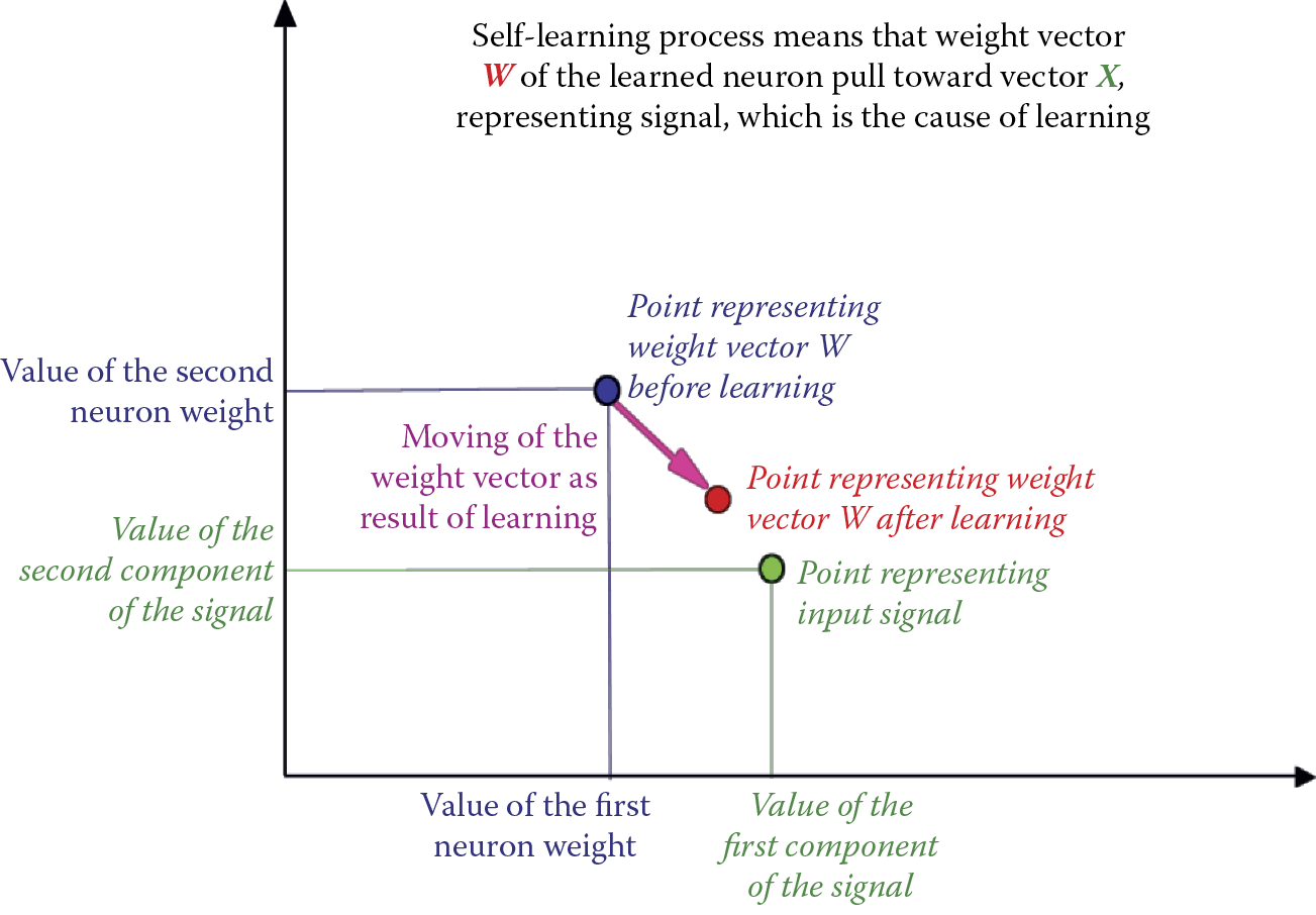
Now let us compare this with self-learning of the winning neuron illustrated in Figure 10.14. Notice that a winner neuron (navy blue point) is subject to teaching because its initial weighting factors were similar to the components of the signal shown during the teaching process (green point). Therefore, amplification and substantiation of only natural (“innate”) neurons occur. The preferences of such neurons were noted in other self-learning networks. The “winner” in the figure was attracted strongly by an input point. Its vector of weights (and a point representing this vector on a figure) will move strongly toward the point representing the input signal.
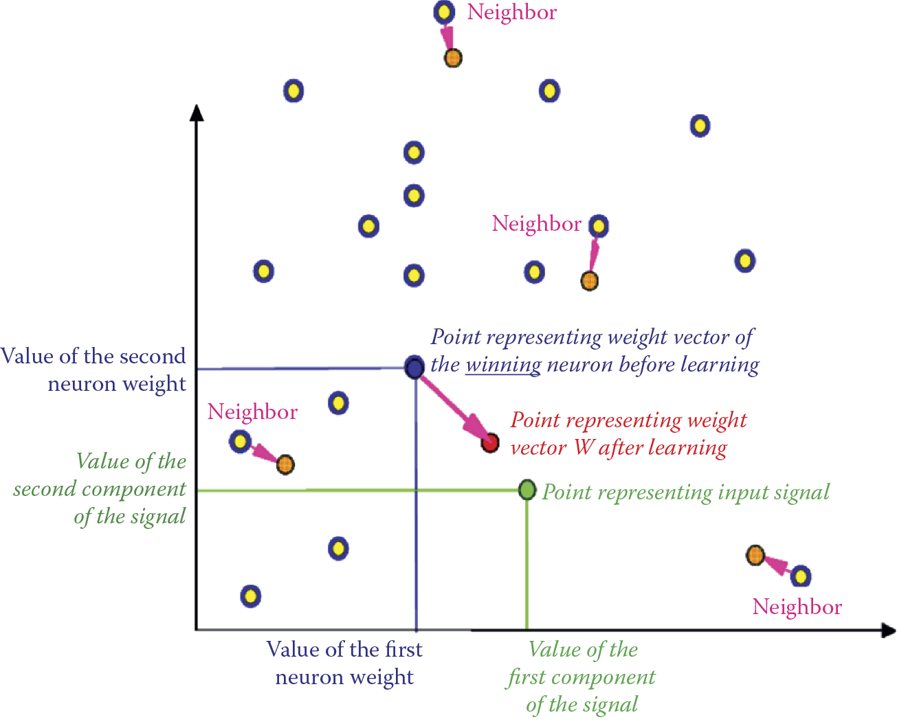
Neighbors of a winner neuron (yellow points lightly toned in red) are not so lucky. However, regardless of their initial weights and output signals, they are taught to have tendency to recognize this input signal even though another neuron became the winner. The neighbors are taught slightly less intensively than the winner (arrows indicating magnitudes of their displacements are visibly shorter).
One important parameter defining a network is the coefficient specifying how much less the neighbors should be taught. The neighbors (yellow points) often have much better parameters and tendency to learn (they were much closer to the input point) because they did not undergo initial teaching as the winner did.
What will be the outcome of this strange teaching method? If the input signals arrive in a manner such that clear clusters are formed, the individual neurons will try to occupy (by their vectors of weights) the positions at the centers of the clusters. The adjacent neurons will “cover” the neighbor clusters as illustrated in Figure 10.15. The green dots in the figure represent input signals; red stars correspond with the locations in the same coordinate system of vectors of weights of the individual neurons.

A less desirable situation will occur when input signals are equally distributed in an area of the input signal space as shown in Figure 10.16. In this case, the neurons of the network will have a tendency to share the function of recognizing these signals and each sub-set of signals will have its “guardian angel” neuron. Each such neuron will detect and recognize all signals from only one sub-area (Figure 10.17). Clearly after input of a set of randomly appearing points and systematic teaching, the location of the point representing the winning neuron’s weights will be the central location in the set (Figure 10.18).
Self-learning using uniform distribution of input data presents a difficult task for a neural network.

Localization of weight vectors of self-learning neurons (larger circles) in points of input space. Neurons may represent sub-sets of input signals (small circles) of the same color.

Mutual compensation of pulling from input vectors reacting with weight vector of self-learning neuron located in the center of a data cluster.
As seen in Figure 10.18, when a neuron (represented as usual by its vector of weights) occupies a location in the center of the “nebula” of points it is meant to recognize, further teaching cannot move it from this location permanently. This is because different points that appear in the teaching sequence cause displacements that compensate each other. To reduce “yawing” of a neuron around its final location, a decreasing teaching coefficient is often applied. Therefore, the essential movements that allow a neuron to find its proper location occur early in the process when the teaching coefficient is still large. The points shown at the end of teaching exert weak influences on the positions of neurons. After a time, a neuron fixes its location and never changes it.
Another process occurs during the teaching of a network. The range of neighborhood systematically decreases. After the start of teaching, the neighborhood restricts and tightens at every step. In the end, each neuron is alone and devoid of neighbors (Figure 10.19).
Notice that when teaching is complete, the neurons of the topological layer will portion the input signal space among themselves so that each area of this space is signaled by a neuron. As a consequence of the influence of neighborhood, these neurons will demonstrate the ability to recognize input objects that are close (i.e., similar to the neurons). This feature is convenient and useful because this kind of self-organization is the key to remarkably intelligent applications of networks as self-organizing representations. We discussed examples of this in the early sections of this chapter.
When presenting the results of teaching a Kohonen network, you will encounter one more difficulty. This is worth discussing before you must deal with simulations in practice. When presenting results (changes in locations of points corresponding to specific neurons during learning), you must also watch the adjacent neurons. In Figure 10.14, it was easy to correlate the movements of the winner neuron and its neighbors. The system had only a few points, and identifying neighbors on the basis of the changed color was easy and convenient. During simulations, sometimes you may have to deal with hundreds of neurons, so the dynamic depicted in Figure 10.14 is impossible to expand to a large network. When presenting the activity of a Kohonen network, mapping of neuron positions is often used. The relation of neighborhood is shown in Figure 10.20.
You can see in Figure 10.20 that points corresponding to adjacent neurons are connected by lines. If the points shift as a result of teaching, the corresponding lines shift too. Of course, this should involve all the neurons and relationships of a neighborhood. For maximum clarity in the figure, we show only lines referring to the winner neuron and its neighbors and omitted all other connections. We will demonstrate this in detail for the full network in the Example 11 program.
10.5 Uses of Kohonen Networks
The program for Example 11 depicts the working of a Kohonen network. Before we attempt to use it, a few comments are in order. At the start, the window will allow you to set the network dimensions in both horizontal and vertical directions (Figure 10.21). The network size is your choice. However, to obtain clear results, start with a small network, perhaps 5 × 5 neurons. Such a network is primitive and it will not be useful for dealing with more complex tasks. However, it will learn quickly and allow you to progress to analyzing networks of greater sizes.

The program code imposes no specific limitations for network size. However, the range of inputs for these parameters is restricted from 1 to 100. During the teaching of big networks on a less efficient computer, you must be patient because finalizing teaching of a large network may require performance of several thousand steps.
Besides setting both the network dimensions in the initial window (Figure 10.21), you can also determine the range of numbers from which the initial values of the weight coefficients (range of initial random weights) will be drawn. We propose that you start by accepting the defaults. You can experiment with various values in further experiments to analyze how the “inborn” abilities of neurons forming a network affect its activity.
After determining the network dimensions and range of initial values, we can proceed to the next screen (Figure 10.22) by using the Next button. We can now follow the progress of teaching. In this window, the location of each neuron in the input signal space will be marked with a blue circle. The red lines connecting circles indicate that the neurons are neighbors based on the assumed rules of binding them (Figure 10.20).
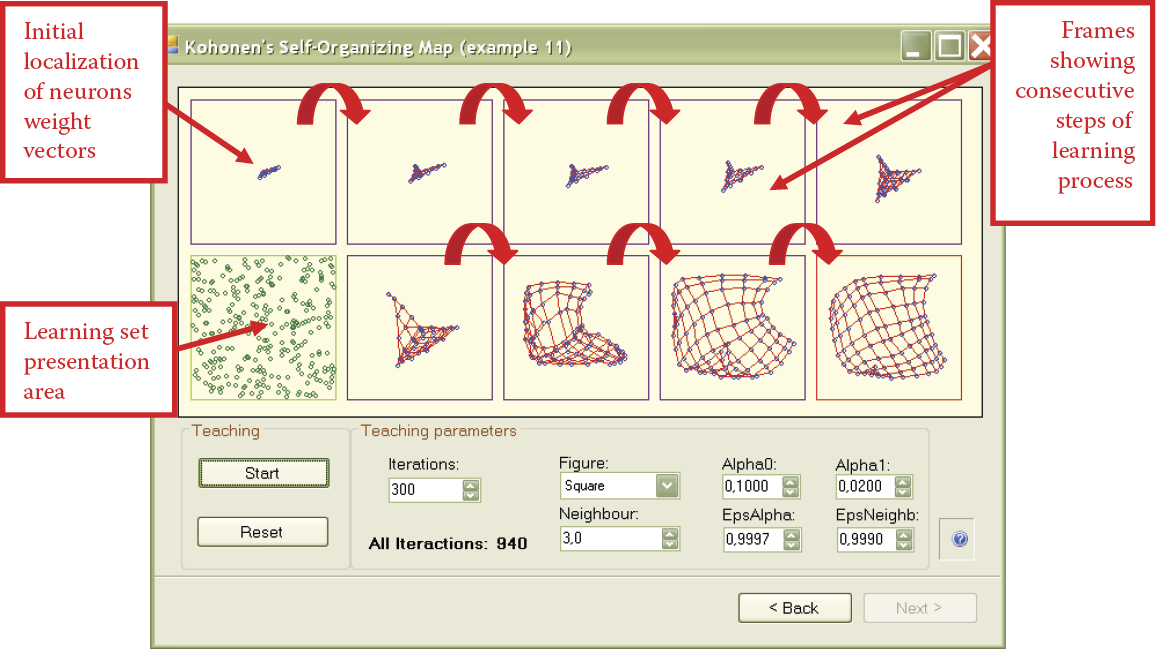
In the input signal space, where the circles are, one neuron recognizes and indicates the appearance of a signal from this point and its close neighborhood (because neural networks always generalize acquired knowledge). The experiments with Kohonen networks usually involve randomly shown points from a certain sub-area of an input signal space. As a result, the blue circles will consequently disperse over the entire input signal space. To be more precise, the teaching signals will be generated from these neurons during teachings. However, these points of input signal space that will not be shown during teaching will not attract neurons.
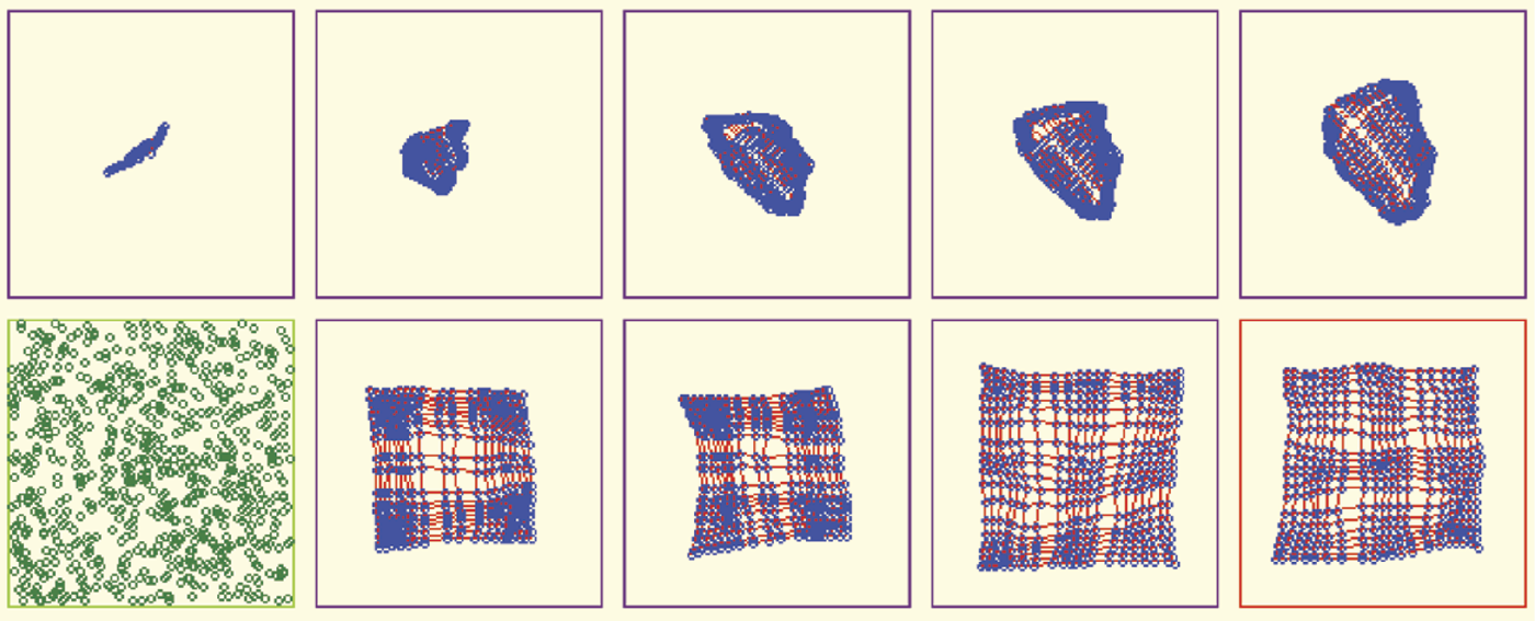
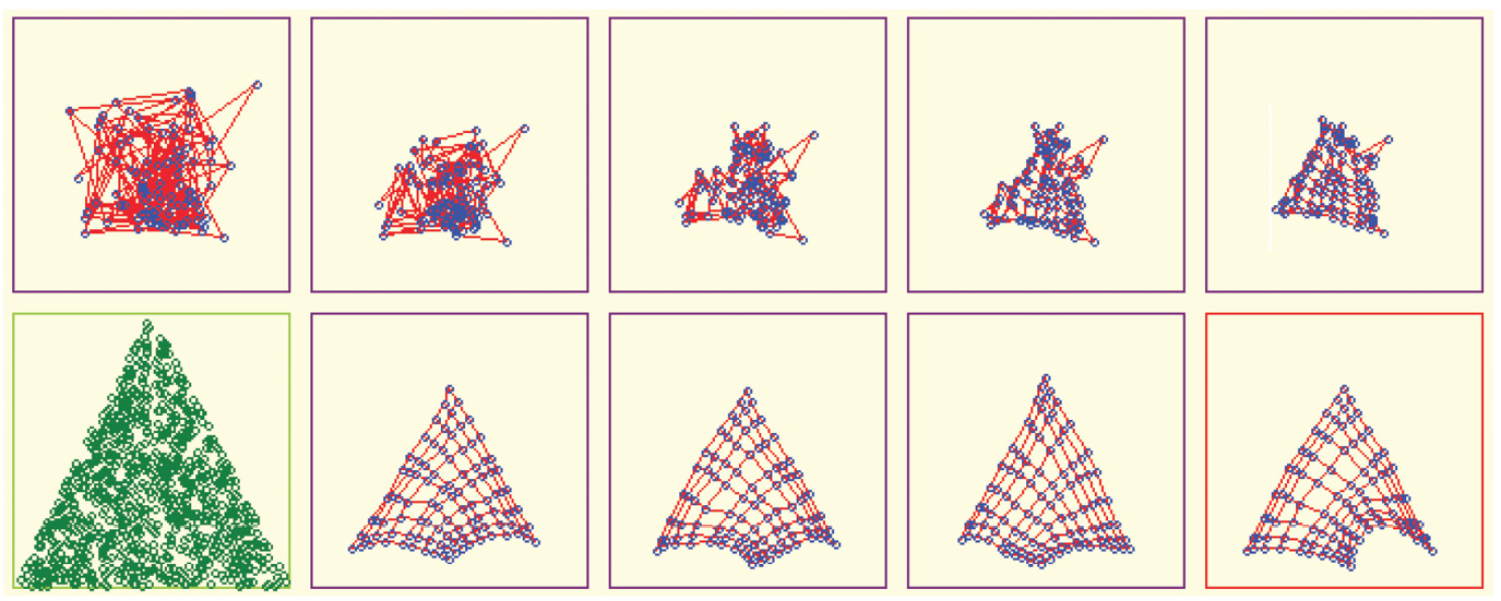
To demonstrate this effect in the Example program, we prepared three options of presenting the training series. Points that teach a network may come from the entire visible area of the input space (this is the “square” option). However, the points may be taken also from the sub-area in the shape of a cross or a triangle. Keep in mind that a network finds representations of only the input signals that are shown in the areas that do not undergo teaching. Generally, not even a single circle representing a neuron “lying in wait” would appear in the area.
After determining the number of steps (iterations) the program must perform, you can use the Figure combination among a group of training parameters to determine the shape of an area. The points recruited to be shown to a network in consecutive phases of teaching will be in this area. The Training Parameters group lists other selections for the self-teaching process.
Pressing the Start button will initialize the network teaching process. The networks of points will appear gradually in the window in the lower left corner (marked by a green frame in the figure) after the count is fixed in the Iterations parameter. All the points have the same color because no teacher has classified them yet. You may notice the sub-space of the input signal space that emits the signals and compare the image with the result of teaching displayed at the end.
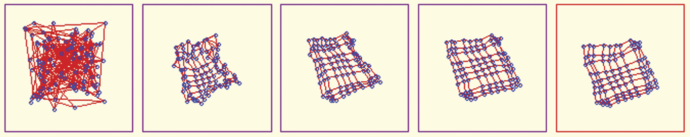
After pursuing the number of steps selected, the program will display a new map showing the distribution of points symbolizing neurons (and their neighborhood relations according to network topology) on the background of the input signal space. The previous map is also visible; the program displays the results of the last few teaching steps. You can monitor the progress of teaching the network. The result of the last training step can be identified easily by the red color of the frame. This is necessary when all the frames will be occupied after many steps of teaching and the screen spaces will be used rotationally.
At the beginning, before the teaching process establishes some order, the neurons occupy somewhat accidental positions in the input signal space. Hence, the blue circles are scattered with no order and the lines connecting the neighbors appear to have no rhyme or reason (Figure 10.23).

As noted earlier, the initial random values are set within the range the user selects. We recommended the use of small initial values of weight coefficients in experiments (e.g., the program suggests 0.01). Usually the unordered cluster of blue circles symbolizing neurons will occupy the densely filled central area of the input signal space.
Although the details will be difficult to see (as in the example in Figure 10.22), we wanted you to see the initial network state before the start of the simulation of teaching. This initial state is shown in Figure 10.23. We set a value of 7 for a scope of random initial weights. We wanted to demonstrate the chaotic initial state of a network, particularly the lines representing the neighborhood.
After every display of neuron location, you may change the number of steps that must be completed before a new point map is generated. It is advisable to use the default values initially. When you understand the workings of the program, you can experiment by changing the number of steps between the consecutive presentations of teaching results. You will note that teaching consisting of dozens or hundreds of steps will produce major changes in the display. If the progress after a segment of teaching is minimal, you may want to use larger jumps (100 or 300 steps) to improve the process, but keep in mind that larger networks mean longer waits to see results.
The intent of this section is to examine the self-organization capability of Kohonen network. We will first investigate the process with simple cases. When teaching starts, a modeling program will activate and show the network points originating from various parts of an input signal space. You can follow the process. The lower left corner of the window will show an area where points shown to the network are displayed (Figure 10.22). You will see the formation of blue circles representing the weights of neurons. These circles at first appear completely chaotic but they will move gradually and distribute equally throughout the input signal space.
You can also view the impact on their locations exerted by neighborhood relations. The red lines indicating which neurons are neighbors will form a systematic mesh and the mesh is subject to expansion. As a result, the vectors of weights of neurons from a topological layer will move so that each of them takes a position that is a centroid (pattern) for some fragment of the input signal space. This process is described as the Voronoi mosaic.
For purposes of this book, we can assume that neurons forming a network step by step specialize in detecting and signalizing different groups of input signals. As a result, after every input signal appears often enough, one neuron in the network will specialize in detecting, signalizing, and recognizing it. In the initial stage (Figure 10.24), the random distribution of points and lines is superseded by an initial ordering of points. The learning process then becomes more subtle and tends to regularize the point distribution.
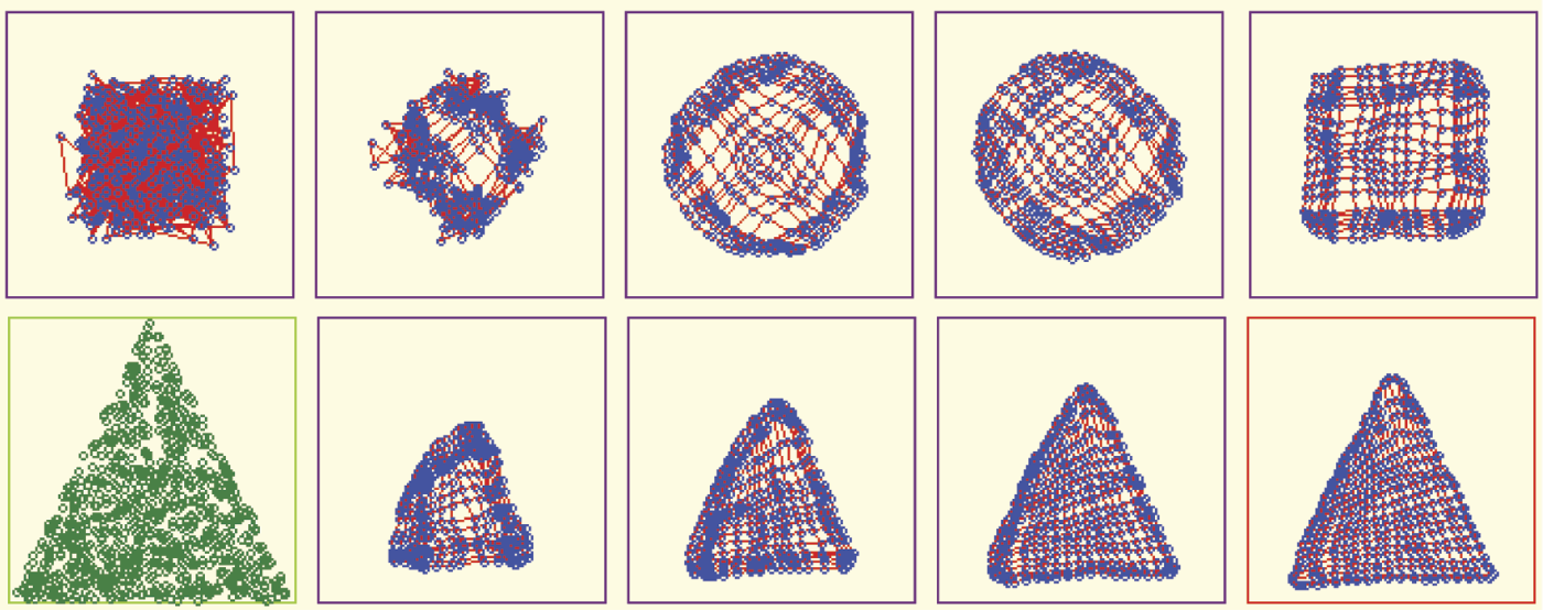
The important issue is that the network creates inner representations in the form of adequate distributions of the values of weight coefficients only for the sub-area of the input signal space where the points were presented originally. Thus, if the input signals come from a limited area (square form in the figure), the Kohonen network tries to cover only this square with the neurons. This occurs with networks having few neurons (Figure 10.25), networks that operate slowly with large numbers of neurons (Figure 10.26), and cases when the initial distribution of neurons takes place in a large area of weight space (Figure 10.27).


Remember that the goal of self-organization always is to have an individual neuron in the network that detects the appearance of a specific point of the input signal space even if the point was not presented during teaching (Figure 10.28).

10.6 Kohonen Network Handling of Difficult Data
The program in Example 11 has superb capability that will enable you to use your imagination to perform several interesting experiments. For example, you can study how a network’s behavior and self-organization are influenced by the method of showing input data. By using the program options, you can demonstrate how the sub-area of the input signal space from which values are taken in a network will be limited even more than the case of squares.
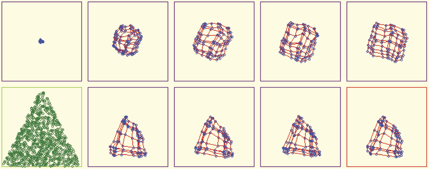
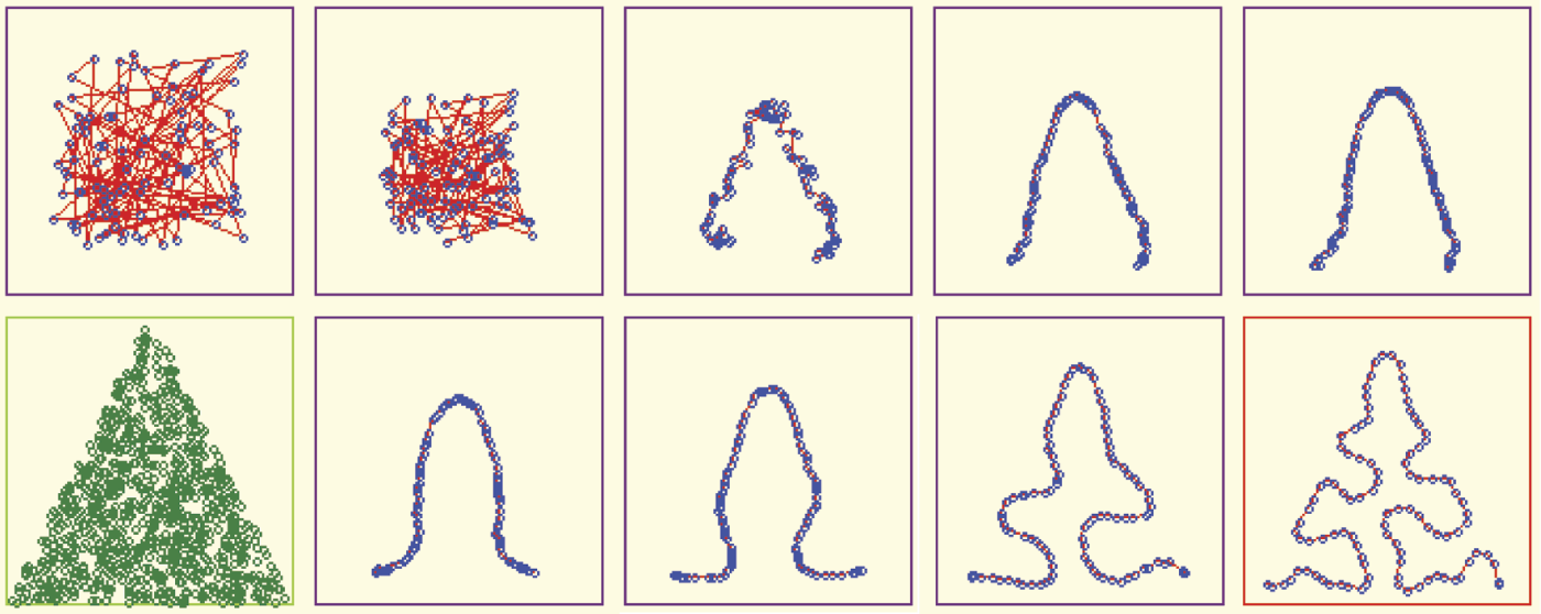
In such a scenario, self-organization tends not to create useless representations of input data. You can observe this phenomenon by providing appropriate input signals to the network. The signals must be chosen from some sub-area of input signal space (e.g., the shape of a triangle). The program will show how all neurons position themselves to recognize all the points inside the triangle (Figure 10.29). No neuron will specialize in recognizing input signals from the space beyond the triangle. Such points were not shown during teaching, so the neurons assume they do not exist and do not have to be recognized.
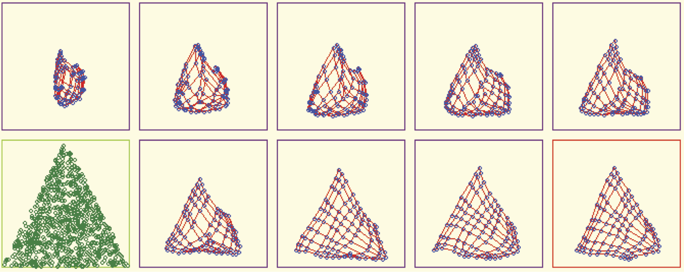
Self-organization where data presented during learning are taken from sub-area (triangle) of input space.
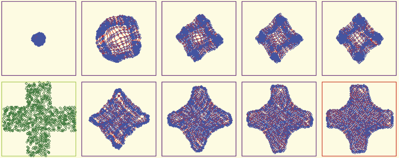
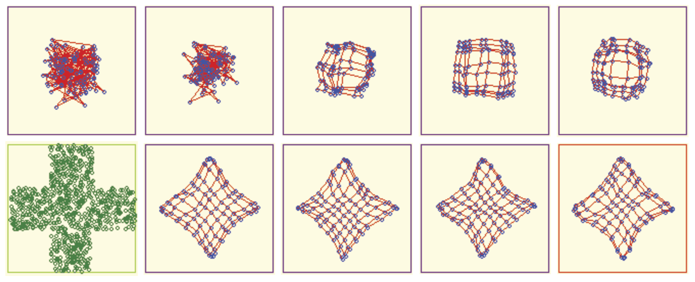
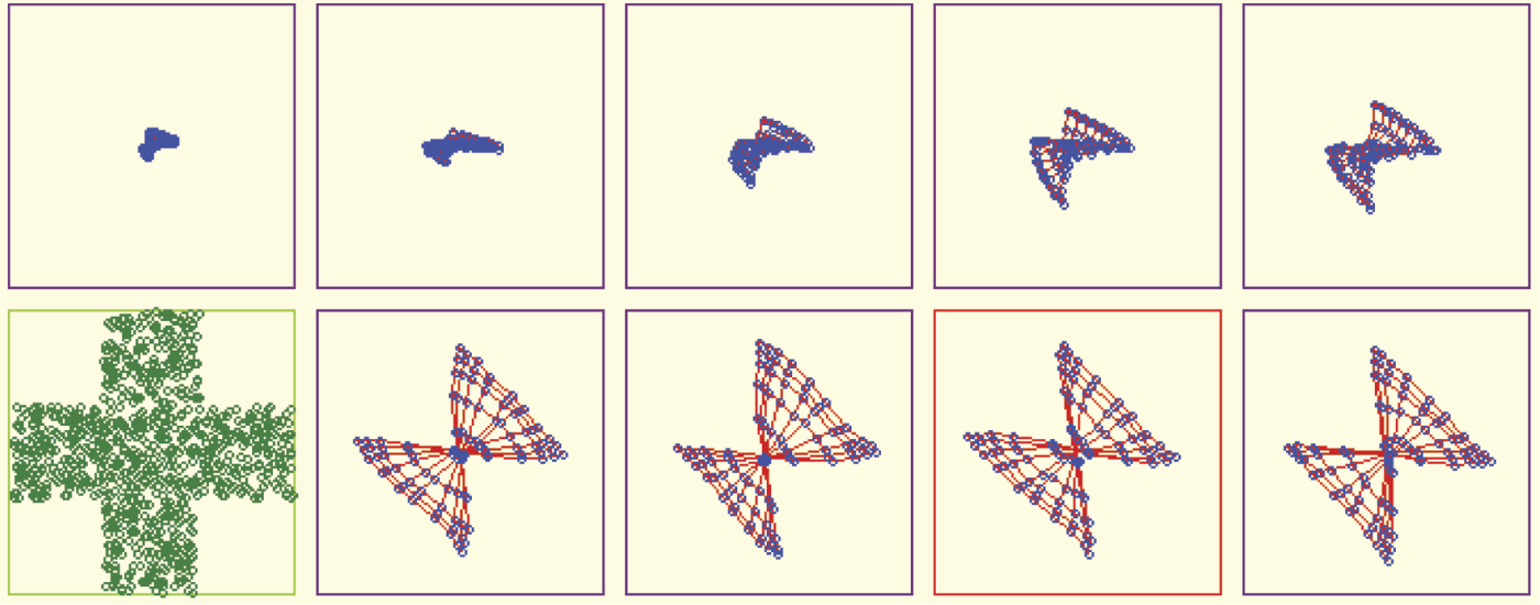
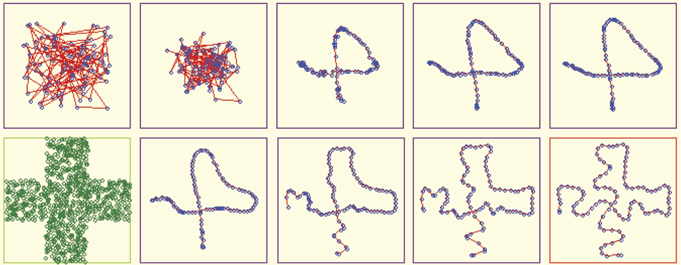
A little more difficult task for a network to fulfill is a more complex form (e.g., a cross) chosen as a sub-area of input signal space. At the start of teaching, the network will be unable to find the proper distribution of neurons (Figure 10.30). Usually tenacious teaching can lead to success in such cases (Figure 10.31). However, success is easier to achieve when teaching a network with a larger number of neurons (Figure 10.32).

Unsatisfactory result of self-organizing where input data are randomly taken from input sub-space in the form of a cross.

10.7 Networks with Excessively Wide Ranges of Initial Weights
A large initial spread of weight coefficients of modeled neurons is not a favorable factor for achieving success from self-organization (Figure 10.33). In such cases, omissions can occur despite a long teaching process. A self-organizing network may ignore certain fragments of active areas of input signal space (bottom right corner of the triangle in Figure 10.34).
Network ignores input data (right lower part of input space) when spread of initial values of neuron weights is too large.
After you experiment with the correct functioning of a network, we encourage you to initiate teaching by using very large values of initial random weights (e.g., 5) for a small simple network (e.g., 5 × 5 neurons) to generate results very quickly. You will probably see the common twisting and collapsing (Figure 10.35 and Figure 10.36) that result from initially overloading a Kohonen network. You may want to experiment by producing such phenomena and determining self-learning cannot lead networks from such “dead ends.”

10.8 Changing Self-Organization via Self-Learning
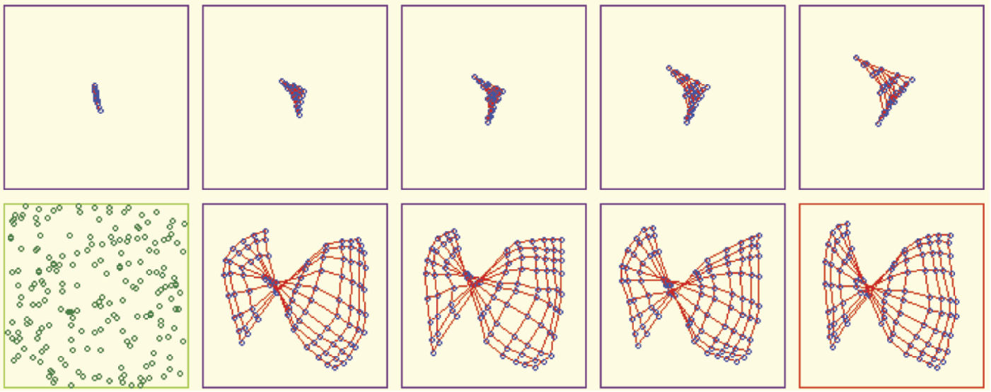
Kohonen networks learn to map their internal memories without intervention from a teacher. They use weight coefficients typically shown as patterns of external (input) signals. You may perform interesting experiments with the Example 11 program. You can change the shape of a sub-area of an input signal space for selecting input data “on the fly.” For example, you can start teaching with a rectangular shape of a sub-area and when the network approaches the desired state, you may change the sub-area shape to a triangle. Figure 10.37 illustrates the results.
You will not always be able to perform such experiments so predictably. Sometimes the final arrangement of a network will contain visible relics of a previously taught figure. Figure 10.38 illustrates the result of abnormal teaching. At first, the network adjusted to the triangular sub-area, then was forced to recognize a rectangular arrangement, and eventually revert to recognizing the triangular shape again.
10.9 Practical Uses of Kohonen Networks
We assume by now that you have a notion of the capabilities of Kohonen networks but what are their real-life practical uses? At the start of this chapter, we described mappings, for example, in robotics that created Kohonen networks spontaneously. If you know how a network works, you will understand this next example. Imagine a robot that has two sensors (because we studied networks that had only two input signals). Let one sensor provide information about the brightness of illumination and the other sense sound volume. This way every point of the input signal space will correspond to a certain environment with specific characteristics (bright and quiet, dark and loud, etc.).
A robot equipped with a Kohonen network starts functioning by observing its surroundings. They may be bright, dark, loud, or quiet. Some combinations of input signals will occur in the robot’s surroundings and others will not. The robot classifies and learns incoming data, specializes its neurons, and after a time has trained its Kohonen network so that every relevant situation corresponds to a neuron that identifies and detects it.
A Kohonen network functions like a robot’s “brain” that reacts to the external world. Humans model such behaviors also. The human brain has neurons that recognize faces, find appropriate routes to various places, select favorite cookies, and avoid a neighbor’s biting dog. The human brain has a model that detects and recognizes every sensory perception and known situation that it encounters. Jerzy Konorski, an outstanding Polish neurophysiologist, associated these internal models of fragments of the outside world with distinct parts of the human brain he called gnostic units.*
Most human perception and ability to recognize conditions of surroundings are based on patterns the brain creates after years of experience in different situations. The patterns are stored in “grandmother cells.” Signals from your eyes, ears, and other senses active these cells (Figure 10.39). Activation considers thousands of models stored in the brain and selects the one that best corresponds to a situation. The capabilities of these cells enable your senses to respond quickly, efficiently, and reliably. However, if your brain fails to develop such models early enough, perception via the senses becomes difficult, slow, and unreliable.
Representation of brain somatosensory stimulus and motion control regions (Source: http://ionphysiology.com/homunculus1.jpg )
Much research supports that conclusion. Most evidence demonstrating the impacts of the external world on internal mechanisms was gathered from animal experiments, for example, studies of sensory deprivation of young cats. Kittens do not develop sight until several days after birth. A group of researchers allowed sighted kittens to see only geometric patterns. Whenever the kittens could have seen other objects, for example, during feeding, the researchers turned off the light.
After a month of such training, the kittens were returned to their normal environment. Kittens who had no sight problems acted like blind animals. They could not see obstacles, food, or even humans because their brains retained only models of geometric figures. Their perception of common objects such as chairs, bowls, and other cats was completely disrupted and long periods of learning were required to enable these cats to regain the ability to see normally.
A similar phenomenon occurs in humans based on studies of anthropologists who observed small-statured Pygmy tribes in Africa. Their natural habitat is dense jungle. The thick vegetation prevented them from seeing long distances. When they were led to open spaces, they completely lost their senses of direction. The simple activity of looking at a distant object left them confused. They reacted to a change of environment such as the approach of an animal as a magical event because their brains lacked models for perceiving events and activities in open spaces.
You may understand how the human brain utilizes internal models of objects by observing daily activities. You can read a newspaper in your native language very easily. If you know the language well, you can scan an article and your brain will turn individual letters into words, words into concepts, and concepts into knowledge. This is possible because many years of learning made your brain adept at reading, developing information, and recalling information later if needed.
A different dynamic occurs when you encounter an unknown word in a text or try to read a message in another language. You may split words into syllables in an effort to understand the meaning but this type of reading is neither easy nor rapid. The reason is that your brain has no ready patterns (models) to relate to the unknown material. This is why archeologists puzzle over inscriptions in unknown ancient languages. If your model of the outside world has no patterns for unfamiliar letters or symbols, you will not understand or remember the material simply because your brain has no gnostic units trained to handle it.
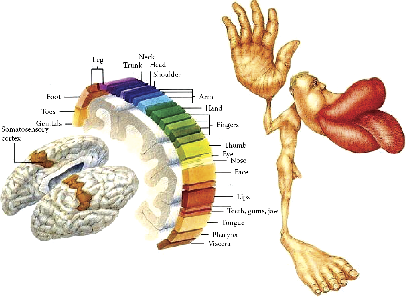
The human brain is capable of creating a map of the body on the surface of the cerebral cortex in the area called the gyrus postcentralis (Figure 10.40). Interestingly, the map does not resemble exactly the shape and proportions of the body. On the surface of a brain, for example, the area mapping the hands and face occupies much more space than the trunk and limbs. This arrangement is analogous to the self-organizing capability of an artificial neural network. Controlling the movements of hands and face and reception of sensory stimuli involves more brain cells because these actions are repeated constantly. In summary, many patterns similar to those in the human brain are created spontaneously in neural networks during the process of self-organizing.

Each area of the body is assigned a proportionate sensory neural area. (Source: http://www.basefields.com/T560/homunculus.htm )
Let us return to the robot example discussed earlier in this section. Every neuron in the robot’s Kohonen network recognizes recurring states of an external world, much like the functioning of gnostic units in the human brain described above. The self-learning process of a Kohonen network creates a specific set of gnostic units (models) within the robot’s controller that are designed to handle every situation the robot may meet. Models are vital because they allow robots and humans to classify every input situation based on signals provided by sensors. After classification of an input into a defined class, a robot may adjust its behavior.
The designer determines what a robot will do in certain situations. For example, in a normal situation, the robot will continue moving forward. It may be programmed to stop if lights are turned off or it hears a noise. The important issue is that the robot does not need constant direction. Its learning is based on the detection of similar situations by a neighborhood of neurons. A trained Kohonen network in a robot brain will figure out what to do.
If a neural network fails to find a ready procedure for a perceived situation, it will determine the closest one based on the neighborhood structure among a set of different states for which proper behaviors have been defined. For example, if a learned action involves forward movement, neighboring situations that are undefined by the user may be applied at reduced speed. If a designer clearly defines actions for a few model situations, a robot will be able to function in most simulation situations, even those not covered by self-learning because of the Kohonen network’s ability to apply averaging and generalization processes.
During teaching, a network may be shown objects (environments) that differ slightly from one another. The objects will be characterized by certain dispersion but the network will remember a certain averaged pattern of input signals in the forms of weight coefficients for certain neurons. The network will involve many typical sample signals and their related environments. The number may be the same as the number of neurons in the network. However, in reality, the system will have fewer neurons than possible environments because the freely changing parameters that characterize a robot’s operations make the number of possible environments infinite.
Through generalization, when a network encounters an environment characterized by parameters not presented during teaching, it will try to fit the environment into a learned pattern. Knowledge gained by a network during learning is generalized automatically, usually producing perfect results.
A robot equipped with a Kohonen network will adapt its behavior to the environment for which it was designed. We know there is a very small commercial market for intelligent mobile robots and thus may wonder about the practical uses for Kohonen networks. In reality, these networks have many applications. For example, banks commonly use these networks to protect against thefts—not thefts involving masked bandits and getaway cars. Modern thefts are more likely to result from fraudulent credit practices. Banks make money by lending money but not all borrowers repay loans. Losses from unpaid loans far exceed losses from armed robberies.
How do banks protect themselves by lending money safely? The answer is simply: building a Kohonen network based on an honest borrower who will repay the principal borrowed and a fair rate of interest, and serve as a standard against which potential new loan applicants are compared.
10.10 Tool for Transformation of Input Space Dimensions
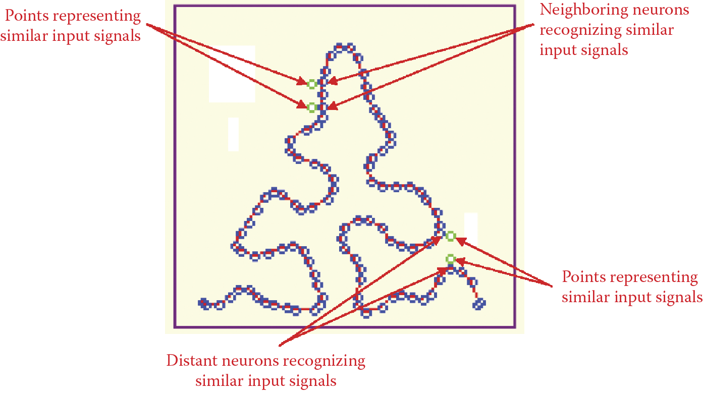
A unique characteristic of a Kohonen network is that it contains a topological representation of an input signal space that applies to neuron neighborhoods. In the illustrations of network actions, blue dots represented neurons and red dots were used to connect adjacent neurons. At the start of example programs, the lines and dots were distributed randomly. During teaching, the network formed orderly arrangements that could be interpreted. Neurons within a network tend to signal and detect adjacent points from an input signal space. As a result, points representing input signals are close together and will be transposed to a network area where adjacent points will be signaled only by adjacent neurons.
In all the figures seen earlier in this chapter, it was easy to associate the notion of similarity of input signals and adjacency (neighborhood) of neurons in a network because input signal space and weight space were two-dimensional (Figure 10.13 and Figure 10.16). The network topology also was two-dimensional (Figure 10.9 and Figure 10.11), thus allowing us to understand such notions as “an input signal lying higher than the previous signal” (higher value of second component) and “an input neuron lying higher than the previous neuron” (in the previous row); see Figure 10.41.
Other situations are possible. We can easily imagine a one-dimensional network that will learn to recognize two-dimensional signals (Figure 10.42). Our program helps you to study the network behavior that makes possible the conversion of a two-dimensional input signal space to a one-dimensional structure using chains of neurons (Figure 10.43).
This unconventional structure may be achieved by giving one dimension of a network (the best is the first one) a value equal to 1. The second dimension should have far greater value (e.g., 100) to ensure it behaves in an interesting way. However, such networks learn quickly so dimensions need not be limited. Figure 10.44 and Figure 10.45 show more examples of such mappings. The figures indicate that one-dimensional networks reasonably fit into the highlighted areas of input signal spaces. This configuration provides two important advantages.

More examples of mapping of two-dimensional input space into one-dimensional neural topology.
Another example of mapping two-dimensional input space into one-dimensional neural topology.
First, a chain of neurons arranged as a one-dimensional network fills the entire selected area of an input signal space. Thus, for every point of two-dimensional input signal space, a representative in a one-dimensional neural network will indicate its occurrence. There are no “orphaned” points or areas in the multidimensional input space.
Second, for objects in an input signal space that lie close (are similar) to each other, the adjacent neurons correspond in the one-dimensional chain of neurons. Unfortunately, although this is likely, it is not guaranteed and you should expect errors (Figure 10.46). However, in most cases, the fact that some states of an input signal space are represented by two adjacent neurons implies that they are similar.
Proper and improper representations of similarities of input signals in neural network topology.
Let us consider the semantics behind this concept. We encounter similar and very difficult problems in many tasks related to informatics. For example, consider the enormous quantities of data required to indicate the complex operations of a nuclear power generating plant. Many hundreds of parameters must be measured and evaluated continuously. Blast furnaces in steelworks, multi-engine aircraft, and manufacturing plants also require effective management of huge amounts of data generated by measurements of thousands of parameters.
We may picture a complex operation as a space involving a great number of dimensions. The result of each measurement (signaling device) should be shown on a separate axis. As certain processes evolve, values of every parameter change and a point corresponding to a state of the considered system changes its position.
Therefore, to estimate the condition of an aircraft, the stability of a reactor, the efficiency of a blast furnace, or company profitability, we need only evaluate the position of a point in a multidimensional space. Specifically, the point represents the state of a parameter and it has a specific meaning, for example, stability of a nuclear reaction or excessive product defects.
To control and inspect a process or product, an engineer or other specialist must have updated and specific information about the process or product including trends of change. To solve such problems in modern engineering, all relevant data are compiled in giant control rooms full of gauges and blinking lights and passed to a person who can make decisions. This procedure is ineffective in practice simply because one individual cannot inspect, control, analyze, and make split-second decisions based on thousands of input data items. In reality, the decision maker does not need such detailed data. He or she needs integrated and well-abstracted global information such as that produced by a Kohonen network.
Imagine that you have built a network in which every neuron gathers thousands of signals. Such a network is more difficult to program than a network with two inputs and also requires more computer memory and more computer time for simulation. Imagine that this network predicts two-dimensional proximities of neurons and the input signal of every neuron will appear at some predetermined point on a screen. Signals of neighbors will be displayed in neighboring rows and columns to indicate their relationships. After teaching a network via Kohonen’s method, you will obtain a tool capable of specific mapping of multidimensional, difficult-to-evaluate data on one screen that may be reviewed and interpreted easily.
Every combination of input signals will be represented by exactly one neuron (winner) that will detect and signal occurrence of this exact situation. If you depict on a screen only an input signal of a specific neuron, you will obtain an image of a moving luminous point. Based on previous experiments, you know which areas of a screen correspond to correct states of a supervised process and which ones indicate unsatisfactory states. By observing the path of the luminous point, you can evaluate system performance.
You can also display output signals of neurons on a screen after introducing competition. You can arrange to have values of output signals displayed in different colors and change parameters to create a colorful mosaic after some practice. What may at first appear as a collection of illegible signals will eventually form an interpretable image.
Other ways exist for depicting results of Kohonen network functioning. However, their one common feature is the use of two-dimensional images because they are relatively easy to interpret. These images do not convey detailed values of data. However, they exhibit synthetic overall images that are valuable to a person who evaluates the results and makes decisions. These images present fairly low levels of data but averaging and generalization techniques described above allow very good results to be obtained. Examples of proper and improper representations of similarity of input signal in neuron network topology are illustrated in Figure 10.47
Example of proper and improper representation of similarity of input signal in neural network topology.
Questions and Self-Study Tasks
1. What is the difference between self-learning and self-organization?
2. Kohonen networks are known as tools that let us look into multidimensional spaces of data. Can you explain this description?
3. One possible application of Kohonen networks is using them as novelty detectors. A network used for this application should signal a set of input signals that never occurred earlier in identical or similar form. Automatic signaling of such situation may have essential meaning (e.g. for detecting a credit card theft or a thief’s use of a cell phone that differs from the way its owner used it). How does a Kohonen network indicate an encounter with a signal with novel characteristics?
4. Study the course of a self-organization process after a change of sub-area of an input signal space from which random input signals come. The space contains a grid created by the network. The program lets you choose one of three shapes (square, triangle, or cross) of a sub-area. Analyze consequences of the choice. If you have advanced programming knowledge, you may devise a program and add more shapes.
5. Study the impact of a coefficient of learning named Apha0 on a neuron. Increases of this coefficient cause acceleration of learning and decreases cause “calming.” If the coefficient is decreased gradually, a learning process that is fast and dynamic at the beginning becomes more stable as time elapses. Change the coefficient and analyze observed results.
6. Study the impact of the changes of a coefficient of learning on neuron neighbors of a winner neuron in a self-organization process. The coefficient is called Alpha1. The higher the Alpha1 value, the more visible the effect when the winner neuron “pulls” its neighbors along. Analyze and describe results of changes of the coefficient value, the Alpha0:Alpha1 ratio, and their impacts on network behavior.
7. Study the impacts of different values of neighborhood range on a network’s behavior and self-organization. This number indicates how many neurons constitute a neighborhood (i.e., how many undergo forced teaching when a winner neuron is self-learning). This number should depend on network size and the default setting. However, we suggest as an exercise a careful examination of its impact on network behavior. Note that larger neighborhood range numbers visibly slow the learning process.
8. Study the impact of changing the EpsAlpha coefficient on self-organization. The EpsAlpha coefficient controls the decreases of Alpha0 and Alpha1 coefficients in every iteration. Note that the smaller the coefficient, the faster the decrease of learning coefficients and the faster learning stabilizes. You can set a value 1 to this coefficient and the learning coefficients will not decrease or set a value slightly more than 1, which will result in more “brutal” learning at every step. Describe the results.
9. Study the impact of changing the range of a neighborhood on network behavior and learning. You can change the EpsNeighb coefficient that controls narrowing (in consecutive iterations) of neighborhood range. Compare the effects of this change to those seen with the EpsAlpha coefficient.
10. Study the effects of over-teaching a network that at first learns to fill a cross-shaped sub-area of an input signal space, then forms a rectangle or triangle. Remember that in over-teaching experiments, you must increase the values of Alpha0 and Alpha1 coefficients and neighborhood range after you change a sub-area.
11. Advanced exercise: Modify the program to model tasks in which a Kohonen network deals with a highly irregular probability of points coming from different regions of an input signal space. Conduct self-learning and you will see that in a taught network, many more neurons will specialize in recognizing signals coming from regions more often represented in a teaching set. Compare the effect with a map of a cerebral cortex (Figure 10.40). What conclusions can you draw from this exercise?
12. Advanced exercise: Write a program simulating the behavior of the robot described in Section 10.9. Attempt to simulate the skills of associating the sensory stimuli describing the environment with behaviors favorable to the robot by causing changes in the environment. Determine the type of representation of knowledge of the robot’s simulated environment to be used and processed by a self-organizing neural network acting as its “brain.” By changing the environmental conditions, determine which conditions the robot can discover in its self-organizing network and which ones are too difficult.
* Konorski J. 1948. Conditioned Reflexes and Neuron Organization. Cambridge, UK: Cambridge University Press.