Streaming Architecture

Because there are so many streaming systems and ways of doing streaming, and everything is evolving quickly, we have to narrow our focus to a representative sample of systems and a reference architecture that covers most of the essential features.

Figure 2-1 shows such a fast data architecture.

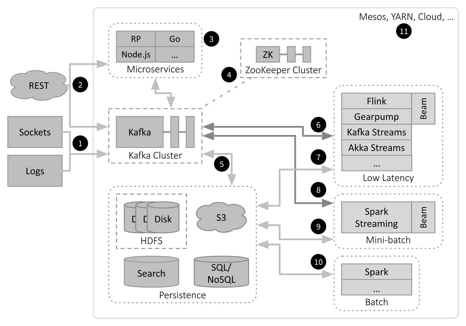
Figure 2-1. Fast data (streaming) architecture

There are more parts in Figure 2-1 than in Figure 1-1, so I’ve numbered elements of the figure to aid in the discussion that follows. I’ve also suppressed some of the details shown in the previous figure, like the YARN box (see number 11). As before, I still omit specific management and monitoring tools and other possible microservices.

Let’s walk through the architecture. Subsequent sections will dive into some of the details:

1. Streams of data arrive into the system over sockets from other servers within the environment or from outside, such as telemetry feeds from IoT devices in the field, social network feeds like the Twitter “firehose,” etc. These streams are ingested into a distributed Kafka cluster for scalable, durable, temporary storage. Kafka is the backbone of the architecture. A Kafka cluster will usually have dedicated hardware, which provides maximum load scalability and minimizes the risk of compromised performance due to other services misbehaving on the same machines. On the other hand, strategic colocation of some other services can eliminate network overhead. In fact, this is how Kafka Streams works,¹ as a library on top of Kafka, which also makes it a good first choice for many stream processing chores (see number 6).

2. REST (Representational State Transfer) requests are usually synchronous, meaning a completed response is expected “now,” but they can also be asynchronous, where a minimal acknowledgment is returned now and the completed response is returned later, using WebSockets or another mechanism. The overhead of REST means it is less common as a high-bandwidth channel for data ingress. Normally it will be used for administration requests, such as for management and monitoring consoles (e.g., Grafana and Kibana). However, REST for data ingress is still supported using custom microservices or through Kafka Connect’s REST interface to ingest data into Kafka directly.

3. A real environment will need a family of microservices for management and monitoring tasks, where REST is often used. They can be implemented with a wide variety of tools. Shown here are the Lightbend Reactive Platform (RP), which includes Akka, Play, Lagom, and other tools, and the Go and Node.js ecosystems, as examples of popular, modern tools for implementing custom microservices. They might stream state updates to and from Kafka and have their own database instances (not shown).

4. Kafka is a distributed system and it uses ZooKeeper (ZK) for tasks requiring consensus, such as leader election, and for storage of some state information. Other components in the environment might also use ZooKeeper for similar purposes. ZooKeeper is deployed as a cluster with its own dedicated hardware, because its demands for system resources, such as disk I/O, would conflict with the demands of other services, such as Kafka’s. Using dedicated hardware also protects the ZooKeeper services from being compromised by problems that might occur in other services if they were running on the same machines.

5. Using Kafka Connect, raw data can be persisted directly to longer-term, persistent storage. If some processing is required first, such as filtering and reformatting, then Kafka Streams (see number 6) is an ideal choice. The arrow is two-way because data from long-term storage can be ingested into Kafka to provide a uniform way to feed downstream analytics with data. When choosing between a database or a filesystem, a database is best when row-level access (e.g., CRUD operations) is required. NoSQL provides more flexible storage and query options, consistency vs. availability (CAP) trade-offs, better scalability, and generally lower operating costs, while SQL databases provide richer query semantics, especially for data warehousing scenarios, and stronger consistency. A distributed filesystem or object store, such as HDFS or AWS S3, offers lower cost per GB storage compared to databases and more flexibility for data formats, but they are best used when scans are the dominant access pattern, rather than CRUD operations. Search appliances, like Elasticsearch, are often used to index logs for fast queries.

6. For low-latency stream processing, the most robust mechanism is to ingest data from Kafka into the stream processing engine. There are many engines currently vying for attention, most of which I won’t mention here.² Flink and Gearpump provide similar rich stream analytics, and both can function as “runners” for dataflows defined with Apache Beam. Akka Streams and Kafka Streams provide the lowest latency and the lowest overhead, but they are oriented less toward building analytics services and more toward building general microservices over streaming data. Hence, they aren’t designed to be as full featured as Beam-compatible systems. All these tools support distribution in one way or another across a cluster (not shown), usually in collaboration with the underlying clustering system, (e.g., Mesos or YARN; see number 11). No environment would need or want all of these streaming engines. We’ll discuss later how to select an appropriate subset. Results from any of these tools can be written back to new Kafka topics or to persistent storage. While it’s possible to ingest data directly from input sources into these tools, the durability and reliability of Kafka ingestion, the benefits of a uniform access method, etc. make it the best default choice despite the modest extra overhead. For example, if a process fails, the data can be reread from Kafka by a restarted process. It is often not an option to requery an incoming data source directly.

7. Stream processing results can also be written to persistent storage, and data can be ingested from storage, although this imposes longer latency than streaming through Kafka. However, this configuration enables analytics that mix long-term data and stream data, as in the so-called Lambda Architecture (discussed in the next section). Another example is accessing reference data from storage.

8. The mini-batch model of Spark is ideal when longer latencies can be tolerated and the extra window of time is valuable for more expensive calculations, such as training machine learning models using Spark’s MLlib or ML libraries or third-party libraries. As before, data can be moved to and from Kafka. Spark Streaming is evolving away from being limited only to mini-batch processing, and will eventually support low-latency streaming too, although this transition will take some time. Efforts are also underway to implement Spark Streaming support for running Beam dataflows.

9. Similarly, data can be moved between Spark and persistent storage.

10. If you have Spark and a persistent store, like HDFS and/or a database, you can still do batch-mode processing and interactive analytics. Hence, the architecture is flexible enough to support traditional analysis scenarios too. Batch jobs are less likely to use Kafka as a source or sink for data, so this pathway is not shown.

11. All of the above can be deployed to Mesos or Hadoop/YARN clusters, as well as to cloud environments like AWS, Google Cloud Environment, or Microsoft Azure. These environments handle resource management, job scheduling, and more. They offer various trade-offs in terms of flexibility, maturity, additional ecosystem tools, etc., which I won’t explore further here.

Let’s see where the sweet spots are for streaming jobs as compared to batch jobs (Table 2-1).

While the fast data architecture can store the same PB data sets, a streaming job will typically operate on MB to TB at any one time. A TB per minute, for example, would be a huge volume of data! The low-latency engines in Figure 2-1 operate at subsecond latencies, in some cases down to microseconds.

What About the Lambda Architecture?

In 2011, Nathan Marz introduced the Lambda Architecture, a hybrid model that uses a batch layer for large-scale analytics over all historical data, a speed layer for low-latency processing of newly arrived data (often with approximate results) and a serving layer to provide a query/view capability that unifies the batch and speed layers.

The fast data architecture we looked at here can support the lambda model, but there are reasons to consider the latter a transitional model.³ First, without a tool like Spark that can be used to implement batch and streaming jobs, you find yourself implementing logic twice: once using the tools for the batch layer and again using the tools for the speed layer. The serving layer typically requires custom tools as well, to integrate the two sources of data.

However, if everything is considered a “stream”—either finite (as in batch processing) or unbounded—then the same infrastructure doesn’t just unify the batch and speed layers, but batch processing becomes a subset of stream processing. Furthermore, we now know how to achieve the precision we want in streaming calculations, as we’ll discuss shortly. Hence, I see the Lambda Architecture as an important transitional step toward fast data architectures like the one discussed here.

Now that we’ve completed our high-level overview, let’s explore the core principles required for a fast data architecture.